[평범한 학부생이 하는 논문 리뷰] Semantic Image Inversion and Editing using Rectified Stochastic Differential Equations (ICLR 2025)

Project Page : https://rf-inversion.github.io/

RF-Inversion

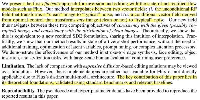
Abstract

본 논문은 rectified flow model의 stochastic 동등성을 이용해서 real image의 inversion과 editing을 다룸

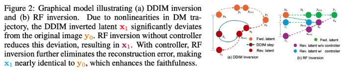
Diffusion Model들의 inversion은 drift와 diffusion에서의 nonlinearity 때문에 faithfulness와 editability에서의 어려움을 제시

본 논문에서는 linear quadratic regulator를 통해 도출된 dynamic optimal control을 사용한 RF inversion을 제시

결과로 나오는 vector field가 rectified stochastic differential equation과 동일하다는 것을 증명

1. Introduction

Vision generative model을 inverting하는 것은 original image를 생성할 수 있는 structured noise를 찾는 것을 포함

Efficient inversion은 다음 두 가지 특성을 만족

• structured noise는 reference image에 faithful한 image를 생성해야 함
• resulting image는 새로운 prompt를 사용해서 쉽게 editable해야함

기존 DM은 이러한 부분에서 널리 사용됐지만, faithfulness와 editability에서 critical challenge를 직면

1. 이 process의 stochastic nature는 reverse SDE의 fine discretization을 필요로 함 → 비싼 Neural Function Evaluation(NFE)를 증가시킴
2. Coarse discretization은 덜 faithful한 output을 생성 (DDIM을 사용해도)
3. Reverse trajectory에서의 nonlinearity는 unwanted drift를 가져옴 → reconstruction의 정확도를 떨굼
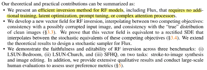
4. Latent variable이나 prompt embedding을 최적화함으로써 기존 방식들은 faithfulness를 강화하지만 이 방식들은 덜 효율적이고 edit하기 더 어렵고 주어진 prompt에 align시키기 위해서 복잡한 attention processor에 의존하는 경향을 가짐 → real-world deployment에 덜 적합함

Inversion과 editing을 위해서, 본 논문은 Rectified Flow(RF)를 사용해서 zero-shot conditional sampling algorithm을 도입

RF는 reverse ODE를 사용해서 효율적인 학습과 빠른 샘플링 모두에서 이점을 가짐

주어진 이미지로 초기화된 controlled forward ODE를 구성해 reverse ODE를 위한 initial condition을 생성

Reverse ODE는 Linear Quadratic Regulator(LQR) 문제를 풀어서 얻은 optimal controller에 의해 guide됨

그 결과로 나온 새로운 vector field는 적절한 drift와 diffusion을 가지는 stochastic interpretation을 가진다는 것을 본 논문에서 증명

2. Method

2.1 Preliminaries

생성모델에서 목표는 target distribution $p_0$에서 유한 개의 sample이 주어졌을 때 이 분포에서 sample을 뽑는 것.

Rectified flow는 ODE를 사용해서 $p_0$를 샘플링하기 위해서 source distribution $q_0$와 time varying vector field $v_t(\mathbf{x}_t)$를 세우는 generative model

• $q_0 \sim \mathcal{N}(0,I)$
• $v_t(X_t) = -u(X_t,1-t;\varphi)$ → $u$는 conditional flow matching objective로 학습된 neural network
• $p_0$ : distribution over images

$X_0 = x_0$로 시작해서 ODE(1)은 $p_0$를 따르는 sample $\mathbf{x}_1$을 생성하기 위해서 $t : 0\rightarrow1$에 대해서 적분

Training Rectified Flows

ODE(1)을 위한 vector field를 제공하는 neural network를 학습시키기 위해서, $p_0$와 $q_0(p_1)$에서의 sample들을 linear path $Y_t = tY_1 + (1-t)Y_0$를 통해 coupling함

$Y_t$의 resulting marginal distribution은 다음과 같음

Initial state $Y_0 = \mathbf{y}_0$와 terminal state $Y_1 = \mathbf{y}_1$가 주어지면, linear path는 ODE를 유도함 : $dY_t = u_t(Y_t | \mathbf{y}_1)dt$ with the conditional vector field $u_t(Y_t|\mathbf{y}_1) = \mathbf{y}_1 - \mathbf{y}_0$

Marginal vector field는 conditional vector field로부터 나옴

다음 flow matching objective를 통해서 neural network로 marginal vector field를 근사 가능

Conditional flow matching objective는 다음과 같음

$\mathcal{L}_{FM}$와 $\mathcal{L}_{CFM}$의 gradient가 동일하고 $\mathcal{L}_{CFM}$이 tractable하기 때문에 학습에 $\mathcal{L}_{CFM}$을 이용

결국 (1)에서 필요로 되는 vector field는 $v_t(X_t) = -u(X_t,1-t,\varphi)$로 계산됨

→ $v_t(X_t) = -u(X_t,1-t,\varphi)$라고 한 이유는 아마 inversion을 $u$로 구하기 위해서인 듯?

이 방식으로 RF는 학습된 vector field를 가지고 ODE로 data distribution에서 샘플링

2.2 Connection between Rectified Flows and Linear Quadratic Regulator

위의 unconditional rectified flow은 random noise의 sample로 초기화된 vector field $v_t(\cdot)$를 simulate함으로써 이미지를 생성 가능

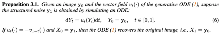
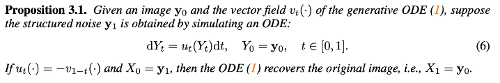
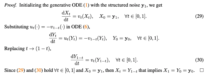
Image로 시작해서 reverse vector field $-v_{1-t}(\cdot)$를 simulate함으로써 시작 noise를 다시 얻을 수 있음

→ 주어진 이미지와의 consistency

Implication

(1)의 vector field를 정확히 알 때, 주어진 이미지의 정확한 inversion이 가능

(6)과 (1)을 사용하면, RF inversion은 정확하게 주어진 이미지를 회복함

 

Corrupted image로 시작해서 reversed vector field $-v_{1-t}(\cdot)$를 simulate한다고 가정

이를 통해 얻어진 noise sample은 두 개의 두드러진 특징이 있음

1. original image와 consistent함 → $v_t(\cdot)$을 통해 처리되면 동일한 corrupted image 생성
2. 만약 image sample이 “atypical”(corrupted or stroke)하면 noise의 sample도 “atypical”

본 논문의 목적은 위 pipeline을 수정해서 corrupted image로 시작해도, clean image를 얻도록 하는 것

이를 위해서 noise sample이 “typical”에 가깝도록 처리 필요

더 일반적으로, 목표는 real image의 semantic editing을 지원하는 pipeline을 만드는 것(without relying on additional training, optimization, or complex attention processors)

첫 스탭으로, 아무 image $Y_0$(손상됐을 수도 있음)를 random noise $Y_1 \sim p_1$(noise that is typical for $p_1$)로 변환하는 minimum energy path를 취하는 optimal controller를 얻음

여기서 $\lambda$는 terminal cost에 할당된 weight, $V(c)$는 control $c : \mathbb{R}^d \times [0,1] \rightarrow \mathbb{R}^d$의 total cost를 나타냄

Control들에 대한 허용 가능한 set에 대한 $V(c)$의 minimization($\mathcal{C}$)은 Linear Quadratic Regulator(LQR) problem이라 알려짐

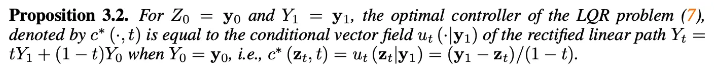
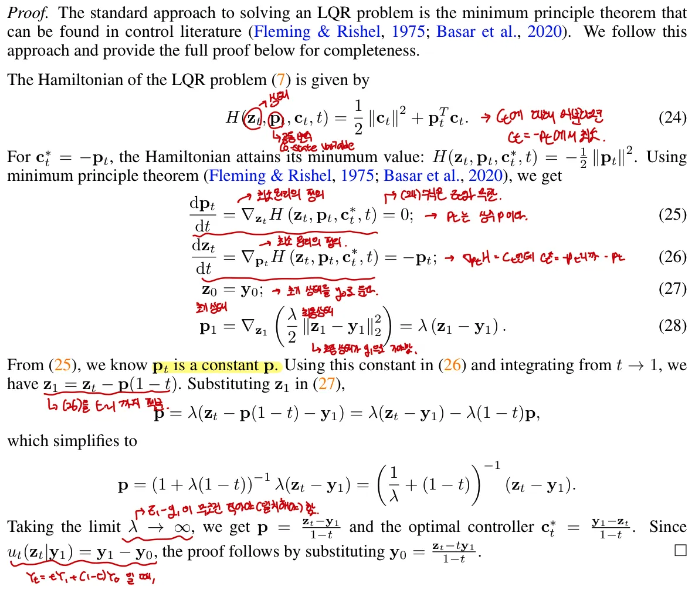
(7)의 해는 다음과 같음

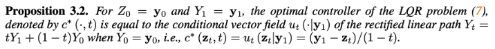
→ image 분포 $p_0$와의 consistency

→ conditional vector field $u_t(\mathbf{z}_t|\mathbf{y}_1)$를 사용하면 corrupted image를 typical noise로 invert가능

2.3 Inverting Rectified Flows with Dynamic Control

위를 통해 두 가지의 vector field를 얻음

1. Proposition 3.1로부터 얻은 vector field → 완벽한 복원이 가능한 vector field
2. Proposition 3.2로부터 얻은 vector field → 손상 됐을 수도 있는 image를 typical한 noise distribution의 sample로 보냄 → (1)을 통해 이미지로 다시 보내면 typical image생성 → $Y_0$(원래 이미지)과 연관은 없음

본 논문의 controlled ODE는 이 두 objective사이의 interpolation으로 정의됨

• $\gamma \in [0,1]$ : tunable parameter인 controller guidance
• $u_t(Y_t) = -v_{1-t}(Y_t)$ : Proposition 3.1
• $u_t(Y_t|\mathbf{y}_1) = c^*(Y_t,t)$ : Proposition 3.2로부터의 insight를 기반으로 계산

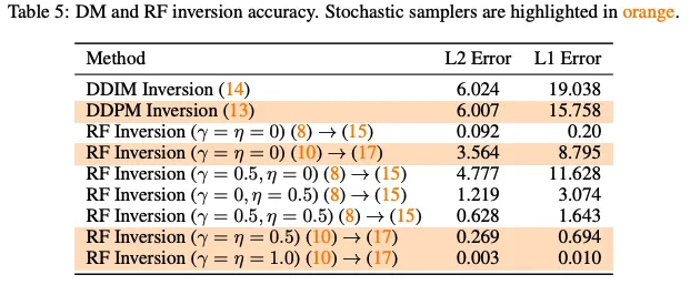
(8)은 inversion accuracy를 유지하면서 (6)를 editing application에 일반화함.

$\gamma =1$이면 (8)은 (7)이 돼서 structured noise $Y_1 = \mathbf{y}_1$가 $p_1$을 준수하도록 함 → (1)을 $\mathbf{y}_1$를 가지고 초기화하면 $p_0$에서 높은 likelihood를 가지는 sample을 생성

$\gamma=0$이면 (8)은 (6)이 돼서 $p_1$을 따르는 것이 보장되지 않는 structured noise $Y_1$를 생성. But, (1)을 이 noise로 초기화하면 image $\mathbf{y}_0$를 정확히 복원

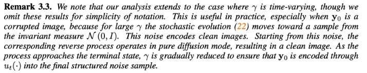
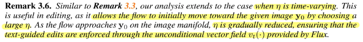
→ $\gamma$를 time-varying으로 할 수 있음

→ 처음에 크게 해서 손상된 이미지를 $\mathcal{N}(0,I)$로 보내고 이 노이즈로 복원하면 clean image로 복원

→ $\gamma$를 점차 줄여서 이미지가 final structured noise sample로 인코딩됨

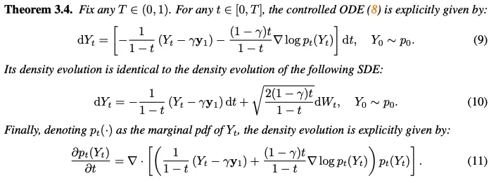
2.4 Controlled Rectified Flows as SDE

SDE가 특정 regularity condition하에서 동등한 ODE formulation을 가진다고 알려져 있음

→ 본 논문에서는 반대로 controlled ODE(8)에 대한 SDE formulation을 보임

(9)의 ODE와 (10)의 SDE는 fokker-planck 방정식에 의해서 (11) 방정식으로 동일하게 변환

Properties of SDE (10)

$\gamma = 0$인 경우, standard RF의 stochastic equivalent가 됨 → Lemma A.2

그 결과 나온 SDE는 다음과 같음

→ image $Y_0$에 대한 faithfulness 향상

$\gamma =1$인 경우, SDE(10)는 LQR problem(7)를 풀고 terminal state $Y_1 =\mathbf{y}_1$로 감

→ 생성 퀄리티를 향상 : sample $Y_1$이 정확한 noise 분포 $p_1$로부터 옴

적절한 $\gamma$의 선택은 원하는 edit을 적용하면서 faithfulness를 가짐

마지막으로 boundary에서의 불규칙성을 피하기 위해 충분히 작은 $\delta$에 대해 $T = 1 -\delta$를 가정

→ Final sample $\mathbf{y}_{1-\delta}$를 $\mathbf{y}_1$로 return

Comparison with DMs

SDE (12)와 유사하게, DMs의 stochastic noising process는 Ornstein-Uhlenbeck(OH) process에 의해 모델링 됨

위 SDE는 다음의 ODE와 대응

→ (13)의 wiener process $W_t$를 $\nabla \rm{log}p_t(Y_t)$로 근사해서 변환

→ Fokker-Planck 방정식으로 변환하면 같아짐

본 논문은 rectified flow를 기초로 함 → 다른 ODE를 이끌고 결국 다른 SDE로 변환됨

Lemma A.1에서 ODE derivation을 formalize함 (ODE를 세움)

Lemma A.2에서 이 ODE의 marginal distribution은 적절한 drift와 diffusion term을 가진 SDE의 marginal distribution과 같음을 보임

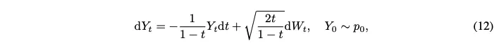
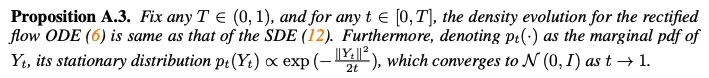
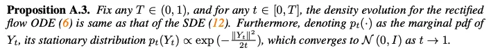
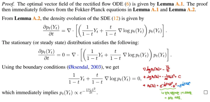
Proposition A.3에서 SDE(12)의 stationary distribution은 $t \rightarrow 1$에 따라 $\mathcal{N}(0,I)$로 수렴

Standard OU process(13)는 $t=0$에서 data distribution과 $t \rightarrow \infty$에서 standard Gaussian 사이를 interpolate

그러나 SDE(12) $t=0$에서 data distribution과 $t=1$에서 standard Gaussian 사이를 interpolate

→ 최종적인 Gaussian distribution을 도달하기 위해 효과적으로 시간을 가속화

이는 (12)에서처럼 time $t$에 의존하도록 drift와 diffusion coefficient들을 수정함으로써 달성

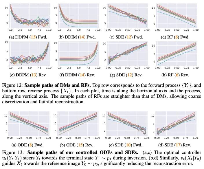
그러므로 (12)의 sample path는 OU process의 것과 다르게 noisy line처럼 보임

2.5 Controlled Reverse Flow using Rectified ODEs and SDEs

위처럼 ODE와 SDE를 reverse 방향(noise to image)으로 develop

Reverse process using ODE

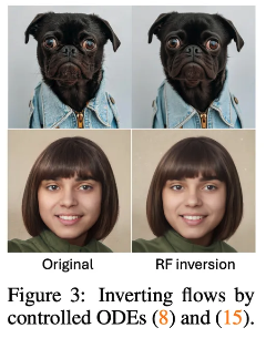
Controlled ODE(8)을 통해 얻은 structured noise $\mathbf{y}_1$에서 시작해서 reverse process를 위한 다른 controlled ODE(15)를 구성. → 이 프로세스에서는 optimal controller는 guidance를 위해 reference image $\mathbf{y}_0$를 사용

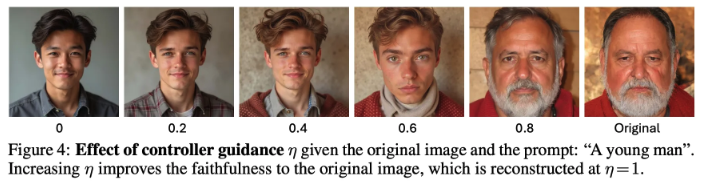
• $\eta \in [0,1]$ : image $\mathbf{y}_0$의 faithfulness와 editability를 control하는 controller guidance parameter

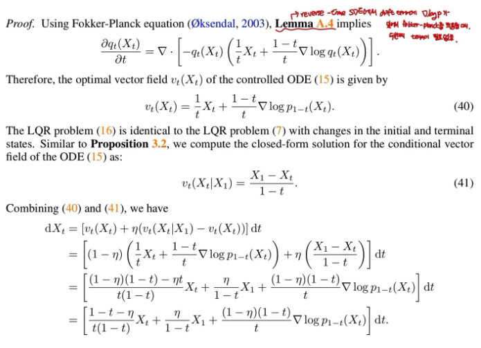
$v_t(X_t|\mathbf{y}_0)$는 수정된 LQR problem(16)을 풀어서 얻어짐

(16)을 풀어서 $c(Z_t,t) = \frac{\mathbf{y}_0 - Z_t}{1-t}$를 얻음

Controller는 sample들이 주어진 이미지 $\mathbf{y}_0$를 향하도록 지시

→ Controlled reverse ODE(15)는 RF model의 standard reverse ODE(1)에 의해 발생하는 reconstruction error를 효과적으로 줄임

Reverse process using SDE

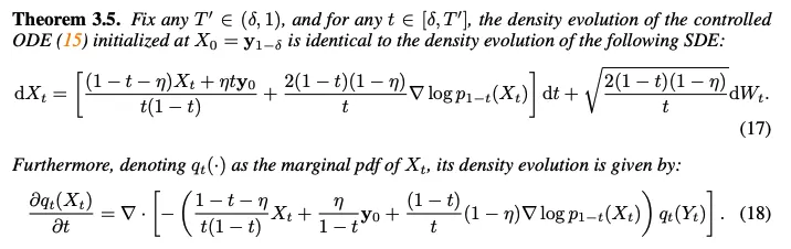
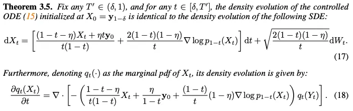
Theorem 3.5에서 controlled reverse ODE(15)의 stochastic equivalent를 제공

→ Controlled forward ODE(8)을 통해 얻은 최종 structured noise로 초기화

Numerical 안정성을 위해서 inversion process를 $T = 1-\delta$에서 종료 → reverse SDE를 $\mathbf{y}_{1-\delta}$에서 시작, 그리고 $T^\prime <1$에서 끝냄

Properties of SDE (17)

$\eta = 0$일 때, pre-trained Flux를 위한 stochastic sampler(22)를 얻음

SDE(17)의 이 경우는 standard RF의 stochastic variant와 상응

본 논문의 key contribution은 inverting rectified flow을 위해서 $X_1 = \mathbf{y}_0$에 대해 conditioning하는 것

본 논문의 explicit construction은 추가적인 학습이나 test-time optimization을 필요로 하지 않음

$\eta=1$일 때, SDE(17)에서 score term과 Brownian motion이 사라져서 drift가 $\frac{\mathbf{y}_0-X_t}{1-t}$됨(LQR problem(16)에 대한 optimal controller) → 주어진 image $\mathbf{y}_0$를 정확히 복원

3. Algorithm : Inversion and Editing via Controlled ODEs

Problem Setup

유저는 reference content를 editing하기 위해서 text prompt를 제공 → 여기서 reference content는 corrupt하거나 clean한 이미지

Corrupt image의 경우

• Reference image는 data distribution $p_0$아래의 realistic image가 아님
• 목표는 original guide에서의 faithfulness를 유지하면서 $p_0$아래의 더 realistic한 이미지로 transform

Clean image의 경우

• Real image $\mathbf{y}_0$와 text prompt 제공
• Content를 보존하면서 $\mathbf{y}_0$에 text-guided edit을 적용

Inversion

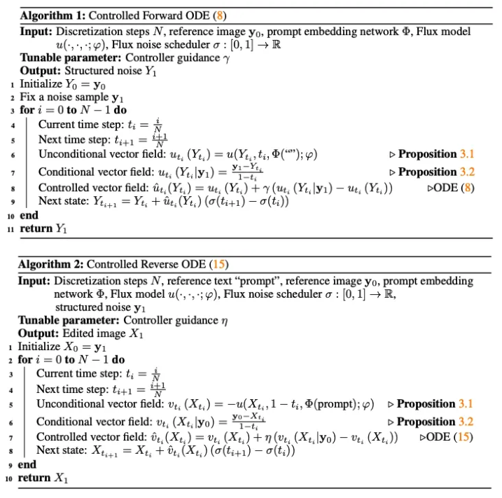
Reference image $Y_0 =\mathbf{y}_0$를 초기조건으로 controlled ODE(8)를 사용해서 structured noise $\mathbf{y}_1$를 계산

Unconditional vector field를 계산하기 위해서 pre-trained Flux model $u(\cdot, \cdot,\cdot ; \varphi)$를 사용 → state $Y_t$, time $t$, prompt embedding $\Phi(\rm{prompt})$를 필요로 함

Inversion process동안에는 null text를 prompt로 사용 → $u_t(\mathbf{y}_t) = u(\mathbf{y}_t,t,\Phi(””);\varphi)$

Conditional vector field를 위해서는 Proposition 3.2에서나온 solution 사용

이 과정을 통해 나온 latent variable은 controlled ODE(15)의 초기 조건으로 사용 → $X_0 = \mathbf{y}_1$

여기서도(reconstruction을 말하는 듯?) null text를 사용 → $v_t = -u(\mathbf{x}_t,1-t,\Phi(\rm{prompt});\varphi)$

Editing

Second step은 reference content $\mathbf{y}_0$의 text-guided editing

이 process는 controlled ODE (15)로 진행됨 → vector field가 Flux로 desired text prompt를 사용해서 계산됨 : $v_t(X_t) = -u(\mathbf{x}_t,1-t,\Phi(\rm{prompt});\varphi)$

(15)에서 controller guidance $\eta$는 faithfulness와 editability의 균형을 맞춤

4. Experiments

Baselines

SoTA inversion 방식들과 비교 : Null-Text Inversion, DDIM inversion, SDEdit

Stroke2Image Generation

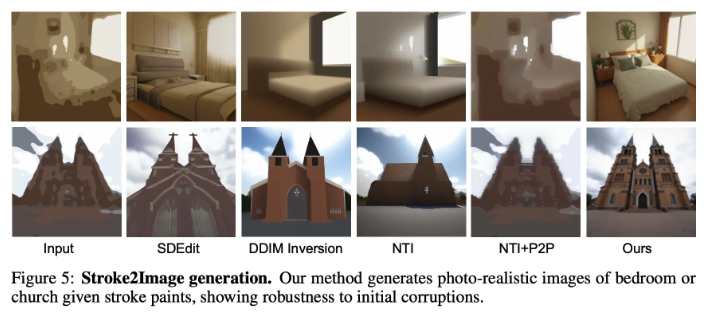
DM inversion들은 stroke painting에서 structured noise로 corruption을 propagate → input stroke painting과 유사한 이미지 생성

Controlled ODE (8)은 corrupted image와 또한 invariant terminal distribution과 일관된 structured noise를 생성 → 더 realistic image를 생성

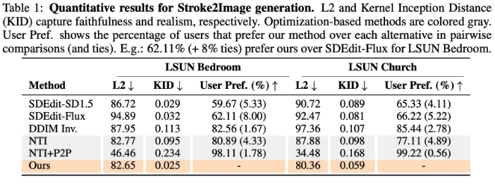
Faithfulness와 realism에서 좋은 성능을 보임

NTI + P2P가 L2 지표에서 크게 좋은 성능을 보이는데, 이는 이 모델이 corrupt image에 가깝게 진행시킴(L2가 낮아짐) → but, image가 unrealistic

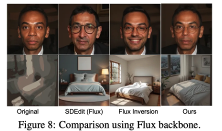
Semantic Image Editing

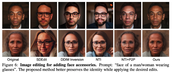
SoTA 방식들과 비교해서 본 논문의 방식은 추가적인 optimization이나 복잡한 attention processor들을 필요로 하지 않음 → 더 효율적임

거기다가 desired edit을 적용하면서 original image에 더 faithful함

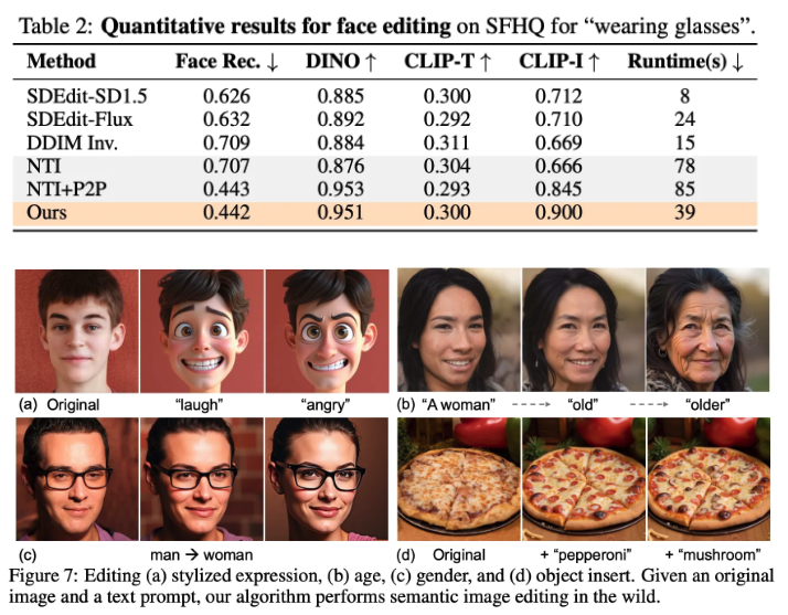
Comparison using the same backbone : Flux

5. Conclusion

A. Additional Theoretical Results

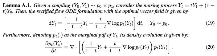
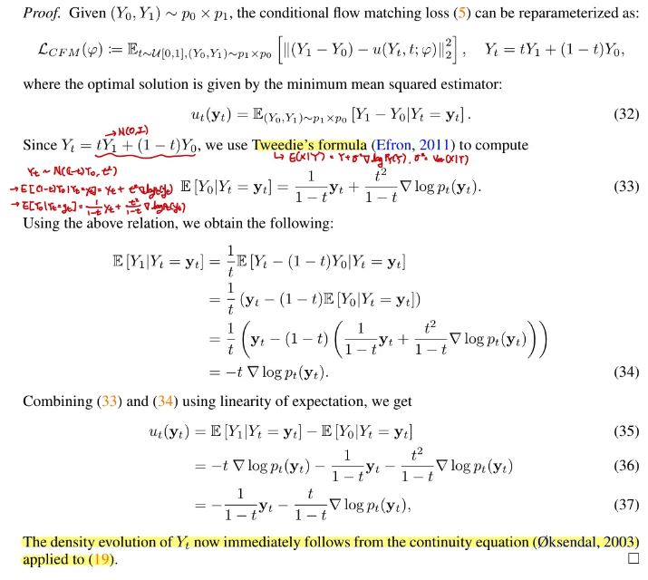
Standard rectified flow(6)를 Lemma A.1 (19)처럼 ODE로 정의함

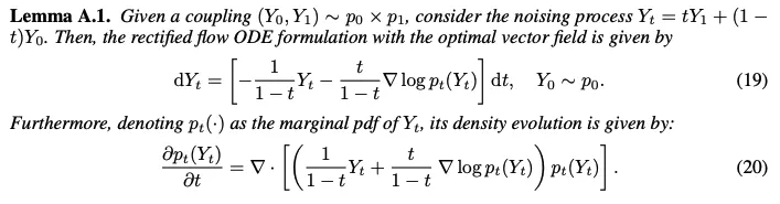
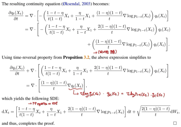
Fokker-Planck equation(continuity equation의 특수한 형태)으로 density evolution가 (20)이 됨

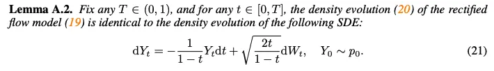
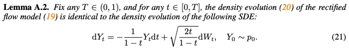
Lemma A.2에 따라 rectified flow(6)의 marginal distribution은 적절한 drift와 diffusion term을 가진 SDE(21)의 marginal distribution과 동일 (density evolution이 동일)

Proposition A.3에 따라, SDE(21)의 stationary distribution은 $t \rightarrow 1$에서 standard Gaussian으로 converge함

위의 lemma들에서 stochastic interpolant formulation을 사용하는 대신, 직접 도출된 명시적인 coefficient들을 제공 (e.g. $\frac{1}{1-t}, \frac{t}{1-t}$)

본 논문의 key contribution은 controlled ODE(8),(15)와 그에 대응하는 equivalent SDEs (10),(17)를 구성한 것

→ faithfulness와 editability를 도움

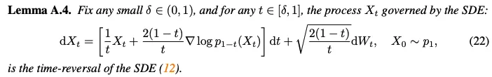
Lemma A.4에서는 rectified flow의 stochastic equivalent(12)를 reverse하는 rectified SDE를 도출(noise를 image로 변환)

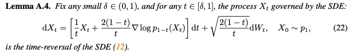
Implication

Reverse SDE(22)는 SoTA rectified flow model을 위한 stochastic sampler를 제공

Score function을 명시적으로 모델링하는 diffusion-based generative model이랑 다르게, rectified flow model은 vector field를 모델링

Vector field $u_t(\mathbf{y}_t)$를 근사하는 neural network $u(\mathbf{y}_t,t;\varphi)$가 주어지면, Lemma A.1은 score function을 계산할 수 있는 명시적인 formula를 제공

SDE(22)의 drift와 diffusion coefficient를 계산하는데 사용 가능.

→ SDE-based sampler가 실용적인 이점이 있는 downstream task에 대한 Flux의 적용성 확장

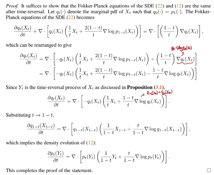
B. Technical Proof

B.1 Proof of Propostion 3.2

B.2 Proof of Proposition 3.1

B.3 Proof of Theorem 3.4

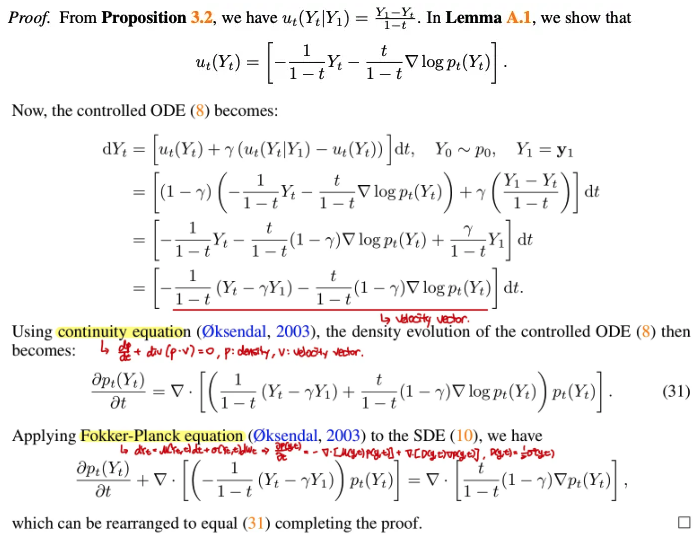
→ controlled ODE(8)와 SDE(10)을 통해 얻은 density evolution이 동일!

B.4 Proof of Lemma A.1

B.5 Proof of Lemma A.2

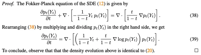
→ (12)와 (19)가 같은 SDE임

B.6 Proof of Proposition A.3

B.7 Proof of Theorem 3.5

B.8 Proof of Lemma A.4

C. Additional Experiments

Algorithm

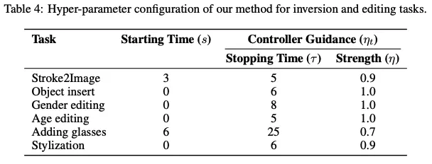
C.1 Hyper-parameter Configurations

Controlled forward ODE(8)에 대해서는 $\gamma = 0.5$ fix

Controlled reverse ODE(15)에 대해서는 time-varying guidance parameter $\eta_t$

C.2 Ablation Study

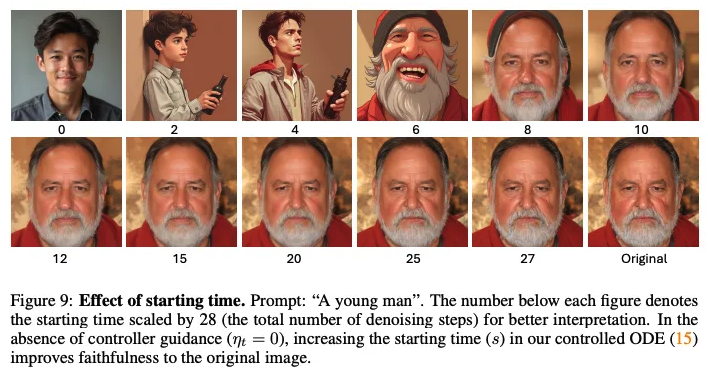
Starting time $s$의 inversion의 faithfulness에 대한 효과

Stopping time $\tau$의 효과

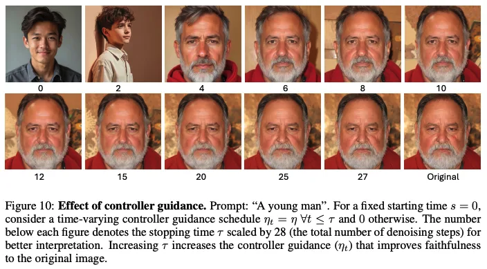
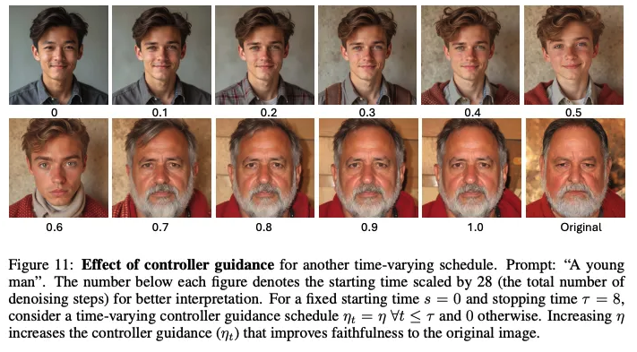
Controll guidance의 효과

C.3 Numerical Simulation

Data distribution : $p_0 = \mathcal{N}(\mu,I)$

Source distribution : $q_0 = \mathcal{N}(0,I)$