
| 일 | 월 | 화 | 수 | 목 | 금 | 토 |
|---|---|---|---|---|---|---|
| 1 | 2 | 3 | 4 | 5 | 6 | 7 |
| 8 | 9 | 10 | 11 | 12 | 13 | 14 |
| 15 | 16 | 17 | 18 | 19 | 20 | 21 |
| 22 | 23 | 24 | 25 | 26 | 27 | 28 |
- visiontransformer
- Python
- 3d generation
- image generation
- image editing
- BOJ
- Programmers
- video generation
- unlearning
- flow matching models
- diffusion models
- rectified flow
- VirtualTryON
- diffusion model
- inversion
- Concept Erasure
- Machine Unlearning
- 프로그래머스
- diffusion
- 코테
- ddim inversion
- rectified flow matching models
- 3d editing
- memorization
- video editing
- 네이버 부스트캠프 ai tech 6기
- flow matching
- rectified flow models
- flow models
- 논문리뷰
- Today
- Total
평범한 필기장
[평범한 학부생이 하는 논문 리뷰] Flow Straight and Fast : Learning to Generate and Transfer Data with Rectified Flow (ICLR 2023) 본문
[평범한 학부생이 하는 논문 리뷰] Flow Straight and Fast : Learning to Generate and Transfer Data with Rectified Flow (ICLR 2023)
junseok-rh 2025. 3. 21. 22:34Paper : https://arxiv.org/abs/2209.03003
Flow Straight and Fast: Learning to Generate and Transfer Data with Rectified Flow
We present rectified flow, a surprisingly simple approach to learning (neural) ordinary differential equation (ODE) models to transport between two empirically observed distributions π_0 and π_1, hence providing a unified solution to generative modeling
arxiv.org
Abstract
본 논문은 경험적으로 관찰된 두 분포 $\pi_0,\pi_1$ 사이를 이동하는 (neural) ODE model을 학습시키는 간단한 approach인 rectified flow를 제안한다. 이를 통해, 분포 이동을 포함하는 다양한 다른 task 중에 generative modeling과 domain transfer에 대한 unified solution을 제공한다. Rectified flow의 아이디어는 $\pi_0, \pi_1$로부터 뽑은 가능한 한 많은 point들을 연결하는 straight path를 따르는 ODE를 학습하는 것이다. 이는 간단한 nonlinear least squares optimization problem을 풂으써 달성된다. Straight path는 두 점 사이의 최단 path이기 때문에 선호되고 특별하다. 그리고 time discretization 없이 정확히 simulation될 수 있고, computationally efficient model을 형성한다. 데이터로부터 rectified flow를 학습하는 절차(rectification)은 $\pi_0, \pi_1$의 임의의 coupling을 non-increasing convex transport cost를 가지는 새로운 deterministic coupling으로 바꾼다. 반복적으로 rectification을 적용하는 것은 점점 straight path를 가진 flow의 sequence를 얻도록하고, 이는 inference 단계에서 coarse time discretization으로 정확히 simulation될 수 있다. 특히, image generation과 translation에 대해, 본 논문의 method는 거의 straight flow를 만들어 single Euler discretization step으로도 고퀄리티의 결과를 가져다준다.
1. Introduction

위와 같은 transport map $T$를 학습시키위한 여러 방식이 제안됐지만, 단점이 존재했다. Neural ODEs를 이용한 flow model과 SDE를 이용한 diffusion model과 같은 continuous time process로써 implicit하게 transport plan을 표현함으로써 발전이 만들어졌다. 이러한 모델들에서, neural network는 process의 drift force를 표현함으로써 학습되고 inference동안 process를 시뮬레이션 하는데 numerical ODE/SDE solver가 사용된다. Key idea는 ODEs/SDEs의 수학적인 구조를 사용함으로써, continuous-time model이 minimax나 traditional approximate inference 기술에 의존하지 않고 효율적으로 학습될 수 있다.
GAN과 VAE와 같은 one-step model과 비교해서, continuous-times model의 key drawback은 inference에서 높은 계산 비용이다. 이는 numerical solver를 가지고 ODE/SDE를 풀어야하기 때문에 반복적으로 비싼 neural drift function을 불러오는 것을 필요로 한다.
또한 기존 방식들은, image generation과 domain transfer를 개별로 다룬다. 이러한 것들을 한번에 다루는 framework는 optimal transport(OT)인데, 이는 고차원의 large volume data에서 느리다는 문제를 지닌다. 또한 transport cost가 실제 learning performance와 완벽히 align되지않기 때문에, optimal transport map을 찾는 방식들은 필수적으로 더 좋은 learning performance를 가지지 않는다.
Contribution
본 논문에서는 rectified flow를 제안한다. Rectified flow는 가능한 한 straight line path를 따르면서 $\pi_0$에서 $\pi_1$로 이동시키는 ODE model이다. Recfified flow는 간단하고 scalable unconstrained least squares optimization 절차로 학습된다. 이는 GAN의 instability issue, MLE method의 intractable likelihood, denoising diffusion model의 미세한 hyper-parameter decision을 피한다. Training data로부터 rectified flow를 얻는 절차는 다음과 같은 매력적인 이론적인 특징을 가진다.
- 모든 convex cost $c$에 대해서 non-increasing transport cost를 가지는 coupling을 생성
- Flow의 path를 점점 straight하게 만들고, numerical solver를 사용해 lower error를 발생
본 논문은 purely ODE-based이고 SDE-based 방식들보다 inference time에서 단순하고 빠르다.
Rectified flow는 매우 적은 Euler step으로 simulation됐을 때 고퀄리티의 image generation 결과를 보인다.

2. Method
2.1 Overview
Rectified Flow
$X_0 \sim \pi_0, X_1 \sim \pi_1$가 주어지면, $(X_0, X_1)$로부터 유도된 rectified flow는 time $t \in [0,1]$에 대한 ODE이다.

Drift force $v : \mathbb{R}^d \rightarrow \mathbb{R}^d$는 $X_0, X_1$로부터 linear path 방향 $(X_1 - X_0)$를 가능한한 따르도록 다음 least square regression 문제를 풀어 설정된다.

단순하게, $X_t$는 $dX_t = (X_1 - X_0)dt$의 ODE를 따른다. 이는 $X_t$의 update가 final point $X_1$의 정보를 필요로하기 때문에 non-causal하다. Drift $v$를 $X_1 - X_0$로 fitting함으로써, rectified flow는 linear interpolation $X_t$의 path를 causalize한다. 이는 미래를 보지 않고 시뮬레이션될 수 있다.
실제로, 본 논문에서는 $v$를 neural network나 other nonlinear model을 통해 parameterize하고 off-the-shelf stochastiv optimizer를 통해 (1)을 푼다. $v$를 얻은 후, $\pi_0$에서 $\pi_1$로 transfer하기 위해 $Z_0 \sim \pi_0$로부터 시작해 ODE를 푼다 (반대도 가능). 특히, backward sampling에서 $\tilde{X}_0 \sim \pi_1$로 초기화되고 $X_t = \tilde{X}_{1-t}$로 셋팅된 $d\tilde{X}_t = -v(\tilde{X}_t, t)dt$를 푼다. (1)이 time-symmetric이여서 $X_0,X_1$을 바꾸고 $v$의 부호를 바꾸면 동일한 문제이기 때문에, forward와 backward sampling은 training algorithm에 의해 똑같이 선호된다.
Flows avoid crossing
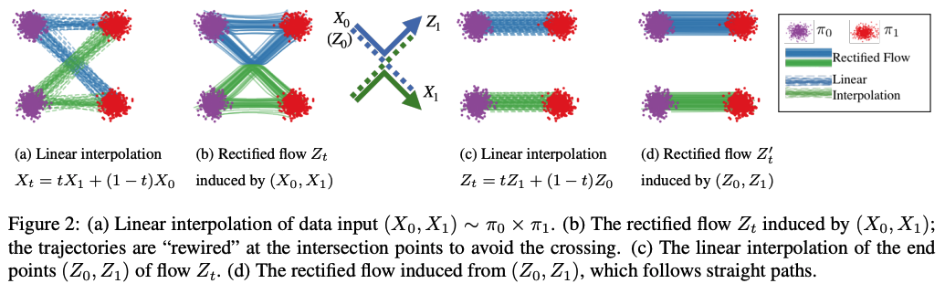
해가 존재하고 유일한 잘 정의된 ODE $dZ_t = v(Z_t,t)dt$를 따르는 다른 path들은 어떤 time $t \in [0,1)$에서도 서로 cross할 수 없다. 구체적으로, 두 path가 $t$에 $z$에서 다른 방향으로 가로지르는 지점 $z$와 시점 $t$가 존재하지 않는다. 그렇지 않으면 ODE의 해가 non-unique하기 때문이다. 반면에, interpolation process $X_t$의 path들은 서로 교차하고 이는 non-causal하게 만든다. Rectified flow는 (1)의 최적화 때문에 linear interpolation path와 동일한 density map을 따르는 반면에, crossing을 피하기 위해서 교차점을 지나는 각 trajectory들을 rewire한다.
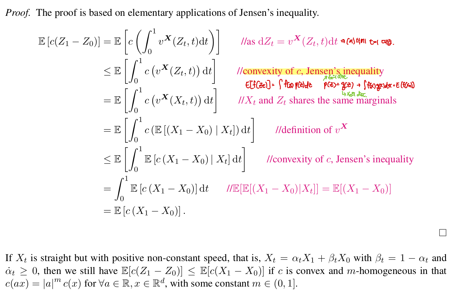
Rectified flows reduce transport costs
만약 (1)이 정확히 풀렸다면, rectified flow의 pair $(Z_0,Z_1)$는 $\pi_0, \pi_1$의 유효한 coupling이라고 보장된다 (Theorem 3.3). 게다가, $(Z_0, Z_1)$은 모든 convex cost functions $c$에 대해서 data pair $(X_0, X_1)$보다 크지 않은 transport cost를 생성한다 (Theorem 3.5). $(X_0, X_1)$은 일반적으로 독립적인 임의의 coupling이다. 반대로, rectified coupling $(Z_0, Z_1)$은 ODE model로부터 구성됐기 때문에 deterministic dependency를 가진다.
Straight line flows yield fast simulation

반복적으로 reflow를 계산하는 것은 $(X_0,X_1)$로부터 유도된 k-rectified flow $\mathbf{Z}^k = \text{RectFlow}((Z^{k-1}_0,Z^{k-1}_1))$를 생성한다. 이 reflow 절차는 transport cost를 감소시킬 뿐만 아니라, rectified flow의 path를 straight하는데 중요한 영향을 가진다.
2.2 Main Results and Properties
Input coupling $(X_0, X_1)$에 대해서, (1)의 정확한 minimum은 다음 수식이면 달성된다.

이는 time $t$에 $x$를 지나는 line direction $X_1 - X_0$의 기댓값이다. 아래에서는 ODE가 unique solution을 가진다고 가정할 때, rectified flow $dZ_t = v^X(Z_t,t)dt \ \text{with} \ Z_0 \sim \pi_0$의 특성에 대해 다룬다.
Marginal preserving property

직관적으로, 이는 (2)에서 $v^X$의 정의에 의해 모든 위치와 시간에서 모든 무한소(infinitesmal) volume을 통과하는 기대 질량은 $X_t, Z_t$의 dynamics하에서 동일하기 때문이다. 이는 동일한 marginal distribution을 추적한다는 것을 보장한다.

한편, $Z_t, X_t$의 전체 trajectory의 joint distribution은 일반적으로 다르다. 특히, $X_t$는 일반적으로 non-causal이고, non-Markovian process이고, $(X_0, X_1)$ stochastic sampling을 가진다. 반면에 $Z_t$는 causalize하고, Markovianize하고 $X_t$를 derandomize한다 (모든 시간에서 marginal distribution을 보존하는 반면).


Reducing transport costs

Transport costs는 하나의 distribution의 질량을 다른 distribution의 질량으로 이동시키는 비용을 측정한다. $\text{Rectify}(\cdot)$는 특정 $c$를 타겟팅하는 것이 아니라 모든 convex transport cost에 대해서 내리는 방향으로 진행된다.
직관적으로, rectified flow $Z_t$의 path는 $(X_0, X_1)$를 잇는 직선 path의 rewiring이기 때문에 convex transport cost가 줄어드는게 보장된다.


Reflow, straightening, fast simulation
아래의 이미지처럼, $\mathbf{Z}^{k+1} = \text{RectFlow}((Z^k_0, Z^k_1))$ 절차를 반복적으로 적용하면 k-rectified flow $\mathbf{Z}^k$의 path가 점점 straight해지고 수치적으로 simulation하기 쉬워진다. 이러한 straightening tendency는 이론적으로 보장된다.

구체적으로, 본 논문에서는 거의 확실하게 $Z_t = tZ_1 + (1-t)Z_0 \ \text{for} \ \forall t \in [0,1]$이거나 동등하게 $v(Z_t, t) = Z_1 - Z_0 = \text{const}$인 경우 flow $dZ_t = v(Z_t,t)dt$는 straight하다고 한다. (더 정확하게 "straight"는 constant speed로 straight하다를 의미) 이러한 straight flow는 효과적인 one-step model이기 때문에 computationally high attractive하다 : a single Euler step update $Z_1 = Z_0 + v(Z_0,0)$가 $Z_0$으로부터 정확한 $Z_1$을 계산한다. $v$가 무조건 inviscid Burgers' equation $\partial_t v + (\partial_z v )v = 0$을 만족해야하기 때문에 flow $dZ_t = v(Z_t,t)dt$를 straight하게 만드는 건 쉽지 않다.

→ 시간에 따른 속도 변화량이 0이라 straight.
더 일반적으로, 다음을 통해 straightness를 측정한다.

$S(\mathbf{Z}) = 0$은 exact straightness를 의미한다.

Figure 1에서 볼 수 있듯이, 한번의 reflow를 적용하는 것이 거의 straight flow를 제공해 single Euler step으로 시뮬레이션할 때 좋은 performance를 보인다. $v^X$에 대한 estimation error를 accumulate할 수도 있기 때문에 너무 많은 reflow step은 추천되지 않는다.
Distillation
k-rectified flow $\mathbf{Z}^k$를 얻고 나서, flow를 시뮬레이션하지 않고 $Z^k_0$으로부터 $Z^k_1$를 바로 예측하기 위해 neural network $\hat{T}$에 $(Z^k_0, Z^k_1)$의 관계를 distill함으로써 inference speed를 향상시킨다. $\hat{T}(z_0) = z_0 + v(z_0,0)$라 하면, $\mathbf{Z}^k$를 distill하기 위한 loss는 $\mathbb{E}[\Vert (Z^k_1 - Z^k_0) - v(Z^k_0,0)\Vert ^ 2]$이다.
Distillation은 충실하게 coupling $(Z^k_0, Z^k_1)$를 근사하려하고, rectification은 lower transport cost와 more straight flow를 가진 다른 coupling $(Z^{k+1}_0,Z^{k+1}_1)$를 생성한다.
On the velocity field $v^X$
$X_1 = x_1$로 condition됐을 때, $X_0$가 conditional density function $\rho(x_0|x_1)$를 생성하면, optimal velocity field $v^X(z,t) = \mathbb{E}[X_1 - X_0 | X_t = z]$는 다음과 같이 표현될 수 있다.

여기서 $\mathbb{E}[\cdot]$은 $X_1 \sim \pi_1$에 관한 것이다. $X_t = z$로 condition됐을 때, $X_0 = \frac{z-tX_1}{1-t}, X_1 - X_0 = \frac{X_1 - z}{1-t}$로 나타냄으로써 보여질 수 있다. 게다가, $\rho$가 모든 곳에서 positive하고 continuous하면, $v^X$는 잘 정의되고 $\mathbb{R}^d \times [0,1)$에서 연속이다. 게다가 $\text{log}\eta_t$가 $z$에 대해서 연속적으로 미분가능하면, 다음을 보일 수 있다.

$v^X$가 $[0,a] \text{ for any } a < 1$에 대해서 uniformly Lipschitz continuous하면, $dZ_t = v^X(Z_t,t)dt$가 유일한 solution을 가진다고 보장된다.
만약 $X_0 | X_1 = x_1$가 conditional density function을 생성하지 않으면, $v^X(z,t)$는 undefine되거나 discontinuous할 수 있고, 이는 ODE $dZ_t = v^X(Z_t,t)dt$가 잘못 작동되게 한다. 간단한 해결책은 $X_0$에 Gaussian noise $\xi \sim \mathcal{N}(0,\sigma^2I)$를 더해 smoothed variable $\tilde{X}_0 = X_0 + \xi$를 생성하는 것이다. 그리고 rectified flow를 통해 $\tilde{X}_0$을 $X_1$로 transfer한다. 이는 $\pi_0$에서 $pi_1$로 이동시키는 $T(X_0 + \xi)$ 형태의 randomized mapping을 효과적으로 준다.
Smooth function approximation
(4)를 따라, conditional density function $\rho(\cdot|x_1)$이 존재하고 알면, 정확하게 $v^X$를 계산할 수 있다. 그리고 $\pi_1$은 유한 개의 point의 empirical measure이다. 이 경우에, rectified flow는 정확하게 $\pi_1$에 있는 point들을 recover한다. 하지만 대부분의 경우 data를 overfitting하기 때문에 실용적으로 유용하지 않다. Large scale problem의 경우에는 neural network나 non-parametric model과 같은 smooth function approximator로 $v^X$를 fitting하는게 필요하고 유용하다. Low dimensional problem에 대해서는 다음과 같은 $v^X$에 대한 간단한 Nadaraya-Watson style non-parametric estimator가 정확한 rectified flow에 대한 좋은 approximation을 생성할 수 있다.

2.3 A Nonlinear Extension
본 논문에서는 linear interpolation $X_t$가 $X_0, X_1$를 잇는 어떤 time-differentiable curve로 대체되는 rectified flow의 nonlinear extension을 제시한다. 이러한 generalized rectified flow가 여전히 $\pi_0$에서 $\pi_1$로 transport할 수 있지만(Theorem 3.3), 더 이상 convex transport costs를 줄이거나 straightening 효과를 가지나는 것을 보장할 수 없다. Probability flow와 DDIM은 이 프레임워크의 특별 케이스로 볼 수 있다.
$\mathbf{X} = \{ X_t : t \in [0,1] \}$로부터 유도된 (nonlinear) rectified flow는 다음과 같이 정의된다.

$\dot{X}_t$는 $X_t$를 $t$에 대해 미분한 것이다. 다음을 풀어서 $v^\mathbf{X}$를 추정할 수 있다.

Theorem 3.3에 의해서 flow $\mathbf{Z}$는 여전히 $\mathbf{X}$의 marginal law를 보존한다. 그러나 $\mathbf{X}$가 straight하지 않으면. $(Z_0, Z_1)$는 $(X_0, X_1)$에 대한 convex transport cost를 줄이는 것을 보장하지 않는다. 또한 더 중요하게, reflow 절차는 더 이상 $Z_t$의 path를 straighten하지 않는다.
2.3.1 Probability Flow ODEs and DDIM

VP ODE와 sub-VP ODE는 다음과 같이 설정된다.


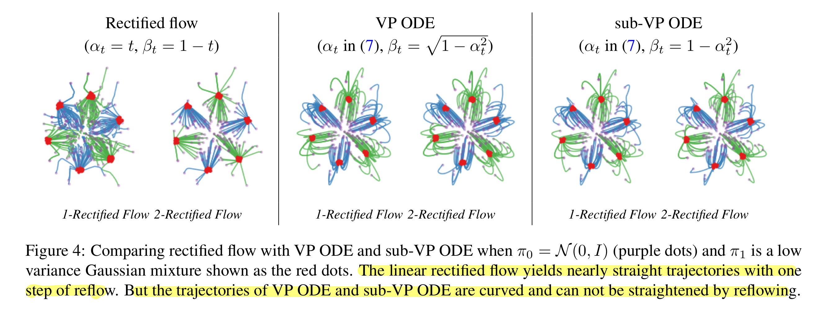

- Non-straight paths : (8)처럼 $\beta_t$를 설정하기 때문에, VP ODE와 sub-VP ODE는 일반적으로 곡선이고 reflow를 통해 straighten되지 않는다.
- Non-uniform speed : (7)처럼 셋팅을 하기 때문에, flow가 처음에는 느리게 움직이고 대부분의 update는 나중에 집중된다.
Summarize


