

| 일 | 월 | 화 | 수 | 목 | 금 | 토 |
|---|---|---|---|---|---|---|
| 1 | 2 | 3 | 4 | 5 | ||
| 6 | 7 | 8 | 9 | 10 | 11 | 12 |
| 13 | 14 | 15 | 16 | 17 | 18 | 19 |
| 20 | 21 | 22 | 23 | 24 | 25 | 26 |
| 27 | 28 | 29 | 30 |
- visiontransformer
- diffusion model
- 논문리뷰
- segmentation map
- 네이버 부스트캠프 ai tech 6기
- Python
- diffusion
- video generation
- rectified flow
- 프로그래머스
- video editing
- Vit
- DP
- diffusion models
- 3d generation
- 3d editing
- inversion
- transformer
- Programmers
- noise optimization
- 코테
- BOJ
- masactrl
- image editing
- flow matching
- segmenation map generation
- memorization
- VirtualTryON
- flipd
- 코딩테스트
- Today
- Total
평범한 필기장
[모델 구현] Vision Transformer 구현 본문
스터디를 통해 Vision Transformer 논문은 읽어봤지만 구현은 해보지 않았었다. 네붓캠 이번주 강의가 DL Basic이여서 Transformer관련 내용도 나오고 코드로 구현하는 실습도 있었다. 그래서 내가 논문 정리해 놓은 것과 연관지어서 코드구현한 것을 포스팅하면 좋을 것 같아서 이렇게 포스팅하게 되었다.
Vision Transformer 논문에 대한 포스팅은 아래 링크에서 볼 수 있다.
https://juniboy97.tistory.com/40
[평범한 학부생이 하는 논문 리뷰] An Image is Worth 16X16 Words: Transformers for Image Recognotion at Scale (ViT)
Transformer 아키텍쳐가 NLP에서 많이 쓰이지만 Vision 분야에서도 쓰인다는 것을 최근에 들었다. Transformer 논문을 최근에 리뷰했는데 이를 Vision 분야에서도 이용한 논문을 읽어봐야겠다는 생각이 들
juniboy97.tistory.com
Vision Transformer Architecture
***이번 포스팅에서의 구현은 Mnist데이터 셋을 기준으로 합니다!!***
ViT의 아키텍처는 아래의 그림과 같다.

Image enbedding
ViT의 input을 보면 input 이미지가 주어지면 크기가 P×P인 패치들로 나누고 각 패치를 flatten시킨다. 이후 linear projection 시킨다. 그리고 각 결과에 이미지의 어느 위치에 있는 패치인지를 나타내기 위해 위치 임베딩을 더해준다. 여기서 분류 task를 위한 모델이기에 class를 나타내는 cls 토큰을 앞에 추가한다. 이 과정의 결과를 수식으로 나타내면 아래와 같다.
z0=[xclass;x1pE;x2pE;⋯;xNpE]+Epos,E∈R(P2⋅C)×D,Epos∈R(N+1)×D(1)
Encoder에 들어가기 전 이미지 데이터를 encoder에 넣기 위해 이미지를 조각으로 나누고 cls 토큰과 각 조각에 위치 임베딩을 더해주어서 encoder에 이미지 데이터를 넣어줄 준비를 과정을 아래 코드처럼 구현할 수 있다.
class image_embedding(nn.Module):
  def __init__(self, in_channels: int = 3, img_size: int = 224, patch_size: int = 16, emb_dim: int = 16*16*3):
    super().__init__()

    self.rearrange = Rearrange('b c (num_w p1) (num_h p2) -> b (num_w num_h) (p1 p2 c) ', p1=patch_size, p2=patch_size)
    self.linear = nn.Linear(in_channels * patch_size * patch_size, emb_dim)
    self.cls_token = nn.Parameter(torch.randn(1, 1, emb_dim))

    n_patches = img_size * img_size // patch_size**2
    self.positions = nn.Parameter(torch.randn(n_patches + 1, emb_dim))

  def forward(self, x):
    batch, channel, width, height = x.shape
    # 원래 input shape : torch.Size([1, 1, 28, 28])

    x = self.rearrange(x) # flatten patches
    # torch.Size([1, 49, 16])

    x = self.linear(x) # embedded patches
    # torch.Size([1, 49, 16])

    c = repeat(self.cls_token, '() n d -> b n d', b=batch)
    # torch.Size([1, 1, 16])

    x = torch.cat((c, x), dim=1)
    # torch.Size([1, 50, 16])


    x = x + self.positions

    return x

emb = image_embedding(1, 28, 4, 4*4)(x)
emb.shape
# torch.Size([1, 50, 16])
rearrrange 함수를 통해 x∈RH×W×C인 input 이미지를 크기가 P×P인 패치들로 나 패치 N개를 각각 x1p∈RP2⋅C로 flatten시킨다. 이후 E∈R(P2⋅C)로 linear projection 시킨다. 그리고 랜덤으로 초기화 된 cls_token을 배치크기로 맞추고 rearrange함수를 거친 input x와 concat시킨다. 그러고 나서 초기화 된 positioning embedding을 더한다.
Encoder
이제는 Transformer Encoder를 구현할 차례이다. 위 이미지에서 오른쪽 이미지가 전체적인 Transformer Encoder를 보여주는데, multi-head self-attention을 먼저 구현해보자.
Multihead self-attention
class multi_head_attention(nn.Module):
    def __init__(self, emb_dim: int = 16*16*3, num_heads: int = 8, dropout_ratio: float = 0.2, verbose = False, **kwargs):
        super().__init__()
        self.v = verbose

        self.emb_dim = emb_dim
        self.num_heads = num_heads
        self.scaling = (self.emb_dim // num_heads) ** -0.5

        self.value = nn.Linear(emb_dim, emb_dim)
        self.key = nn.Linear(emb_dim, emb_dim)
        self.query = nn.Linear(emb_dim, emb_dim)
        self.att_drop = nn.Dropout(dropout_ratio)

        self.linear = nn.Linear(emb_dim, emb_dim)

    def forward(self, x: Tensor) -> Tensor:
        # query, key, value
        Q = self.query(x)
        K = self.key(x)
        V = self.value(x)
        if self.v: print(Q.size(), K.size(), V.size())
        # torch.Size([1, 50, 16]) torch.Size([1, 50, 16]) torch.Size([1, 50, 16])

        # q = k = v = patch_size**2 + 1 & h * d = emb_dim
        Q = rearrange(Q, 'b q (h d) -> b h q d', h=self.num_heads)
        K = rearrange(K, 'b k (h d) -> b h d k', h=self.num_heads)
        V = rearrange(V, 'b v (h d) -> b h v d', h=self.num_heads)
        if self.v: print(Q.size(), K.size(), V.size())
        # torch.Size([1, 4, 50, 4]) torch.Size([1, 4, 4, 50]) torch.Size([1, 4, 50, 4])

        ## scaled dot-product
        weight = torch.matmul(Q, K)
        weight = weight * self.scaling
        if self.v: print(weight.size())
        # torch.Size([1, 4, 50, 50])

        attention = torch.softmax(weight, dim=-1)
        attention = self.att_drop(attention)
        if self.v: print(attention.size())
        # torch.Size([1, 4, 50, 50])

        context = torch.matmul(attention, V)
        context = rearrange(context, 'b h q d -> b q (h d)')
        if self.v: print(context.size())
        # torch.Size([1, 50, 16])

        x = self.linear(context)
        return x , attention

feat, att = multi_head_attention(4*4, 4, verbose=True)(emb)
feat.shape, att.shape
# (torch.Size([1, 50, 16]), torch.Size([1, 4, 50, 50]))
Transformer 논문에서 나온 것 처럼, 일단 query, key, value를 구하고 head의 개수만큼 나눈다. 그런 후 query와 key를 행렬 곱을 시킨 후 scaling시킨후에 soft max 함수에 넣어주어서 attention값을 계산해준다. 그러고 나서 value 값과 행렬곱을 해줘서 output이 나오도록 해서 multihead self-attention을 완성 시켜준다.
이 다음으로 encoder에서 MLP block이 필요하기 때문에 MLP block을 구현해보자.
MLP Block
논문에서 2개의 레이어와 GeLU 활성화 함수를 이용해 MLP block을 만들었다고 하니 그대로 구현해준다.
class mlp_block(nn.Module):
    def __init__(self, emb_dim: int = 16*16*3, forward_dim: int = 4, dropout_ratio: float = 0.2, **kwargs):
        super().__init__()
        self.linear_1 = nn.Linear(emb_dim, forward_dim * emb_dim)
        self.dropout = nn.Dropout(dropout_ratio)
        self.linear_2 = nn.Linear(forward_dim * emb_dim, emb_dim)

    def forward(self, x):
        x = self.linear_1(x)
        x = nn.functional.gelu(x)
        x = self.dropout(x)
        x = self.linear_2(x)
        return x
Transformer Encoder
위에 구현해둔 Multihead self-attention과 MLP block을 이용해서 최종적인 Transformer Encoder를 완성시켜보자.
class encoder_block(nn.Sequential):
    def __init__(self, emb_dim:int = 16*16*3, num_heads:int = 8, forward_dim: int = 4, dropout_ratio:float = 0.2):
        super().__init__()

        self.norm_1 = nn.LayerNorm(emb_dim)
        self.mha = multi_head_attention(emb_dim, num_heads, dropout_ratio)

        self.norm_2 = nn.LayerNorm(emb_dim)
        self.mlp = mlp_block(emb_dim, forward_dim, dropout_ratio)

        self.residual_dropout = nn.Dropout(dropout_ratio)

    def forward(self, x):
        x_ = self.norm_1(x)
        x_, attention = self.mha(x)
        x = x_ + self.residual_dropout(x)

        x_ = self.norm_2(x)
        x_ = self.mlp(x)
        x = x_ + self.residual_dropout(x)
        return x, attention

feat, att = encoder_block(4*4, 2, 4)(emb)
feat.shape, att.shape
# (torch.Size([1, 50, 16]), torch.Size([1, 2, 50, 50]))
Transformer Encoder의 그림을 보면 encoder에 input이 들어오면 layer norm을 거쳐 multihead attention block에 들어가고 이 과정에서 residual connection이 있다. 그러고 나서 또 다시 layer norm을 거쳐 MLP block을 거치고 이 과정에서도 residual connection이 쓰인다. 이 과정을 위 코드처럼 구현을 해놨다.
Model
앞에서 구현한 것들을 가지고 전체적인 모델을 만들어 보자. 일단 전체적인 코드를 보면 아래와 같다.
class vision_transformer(nn.Module):
    def __init__(self, in_channel: int = 3, img_size:int = 224,
                 patch_size: int = 16, emb_dim:int = 16*16*3,
                 n_enc_layers:int = 15, num_heads:int = 3,
                 forward_dim:int = 4, dropout_ratio: float = 0.2,
                 n_classes:int = 1000):
        super().__init__()
        self.image_embedding = image_embedding(in_channel, img_size, patch_size, emb_dim)
        self.transformer_encoder = nn.ModuleList([encoder_block(emb_dim, num_heads, forward_dim, dropout_ratio)for _ in range(n_enc_layers)])

        self.reduce_layer = Reduce('b n e -> b e', reduction='mean')
        # 패치별로 나온 결과 값을 합치는 과정!! ->  패치별로 계산을 했기 때문에 합치는 과정이 필요하다!!
        self.normalization = nn.LayerNorm(emb_dim)
        self.classification_head = nn.Linear(emb_dim, n_classes)

    def forward(self, x):
        x = self.image_embedding(x)
        attentions = []
        for encoder in self.transformer_encoder:
            x, att = encoder(x)
            attentions.append(att)

        x = self.reduce_layer(x)
        x = self.normalization(x)
        x = self.classification_head(x)

        return x, attentions

y, att = vision_transformer(1, 28, 4, 4*4, 3, 2, 4, 0.2, 10)(x)
y.shape, att[0].shape
# (torch.Size([1, 10]), torch.Size([1, 2, 50, 50]))
처음에 설명을 해야할 부분은 transformer_encoder부분인데 ViT도 그렇고 Transformer도 그렇고 encoder가 여러 개 쌓여있는 구조이다. 그렇기에 똑같은 encoder를 하나의 리스트에 넣어서 반복문을 통해 반복해서 계산해 준다. 그리고 reduce_layer같은 경우는 인코더를 통해서 계산돼서 나온 output은 이미지를 패치별로 나누었기 때문에 패치별로 결과가 나온다. 그렇기에 다시 패치들의 결과를 하나로 합치는 과정이 필요하다. 그렇기에 다시 합치는 방식을 지정해 준 것이라고 이해하면 되겠다. ViT는 이미지를 분류하기 위한 모델이기에 마지막으로 classification을 위한 MLP block이 들어가 줘야한다.
이러한 전체적인 과정을 통해 ViT를 구현을 완성했다.
Training & Result
Mnist 데이터셋으로 구현된 ViT모델을 학습시키고 결과를 봤다. Training detail은 아래와 같다.
transform = T.Compose([
                T.ToTensor()
            ])

dataset_train = dset.MNIST('dataset', train=True, download=True, transform=transform)
dataset_test = dset.MNIST('dataset', train=False, download=True, transform=transform)

model = vision_transformer(1, 28, 4, 4*4, 3, 2, 4, 0.2, 10)
model.to(device)

num_epochs = 10
criterion = nn.CrossEntropyLoss()
optimizer = optim.Adam(model.parameters(), lr=1e-3)

batch_size = 64
dataloaders_train = DataLoader(dataset_train, batch_size=batch_size, sampler=sampler.SubsetRandomSampler(range(0, len(dataset_train) * 4//5)))
dataloaders_valid = DataLoader(dataset_train, batch_size=batch_size, sampler=sampler.SubsetRandomSampler(range(len(dataset_train) * 4//5, len(dataset_train))))
dataloaders_test = DataLoader(dataset_test, batch_size=batch_size)
아래와 같이 training을 시켰다.
for epoch in range(num_epochs):
    print('*** Epoch {} ***'.format(epoch))

    # Training
    model.train()
    running_loss, running_acc = 0.0, 0.0

    for idx, (inputs, labels) in enumerate(dataloaders_train):
      inputs = inputs.to(device)
      labels = labels.to(device)

      # zero the parameter gradients
      optimizer.zero_grad()

      # forward
      with torch.set_grad_enabled(True):
        outputs, _ = model(inputs)
        _, preds = torch.max(outputs, 1)
        loss = criterion(outputs, labels)

        loss.backward()
        optimizer.step()

        # statistics
        running_loss += loss.item() * inputs.shape[0]
        running_acc += torch.sum(preds == labels.data)
    running_acc /= (idx+1) * batch_size
    print('{} Loss: {:.4f} Acc: {:.4f}'.format('train', running_loss, running_acc))

    # Validation
    model.eval()
    running_acc = 0.0

    for idx, (inputs, labels) in enumerate(dataloaders_valid):
      inputs = inputs.to(device)
      labels = labels.to(device)

      with torch.set_grad_enabled(False):
        outputs, _ = model(inputs)
        _, preds = torch.max(outputs, 1)

        # statistics
        running_acc += torch.sum(preds == labels.data)
    running_acc /= (idx+1) * batch_size
    print('{} Acc: {:.4f}\n'.format('valid', running_acc))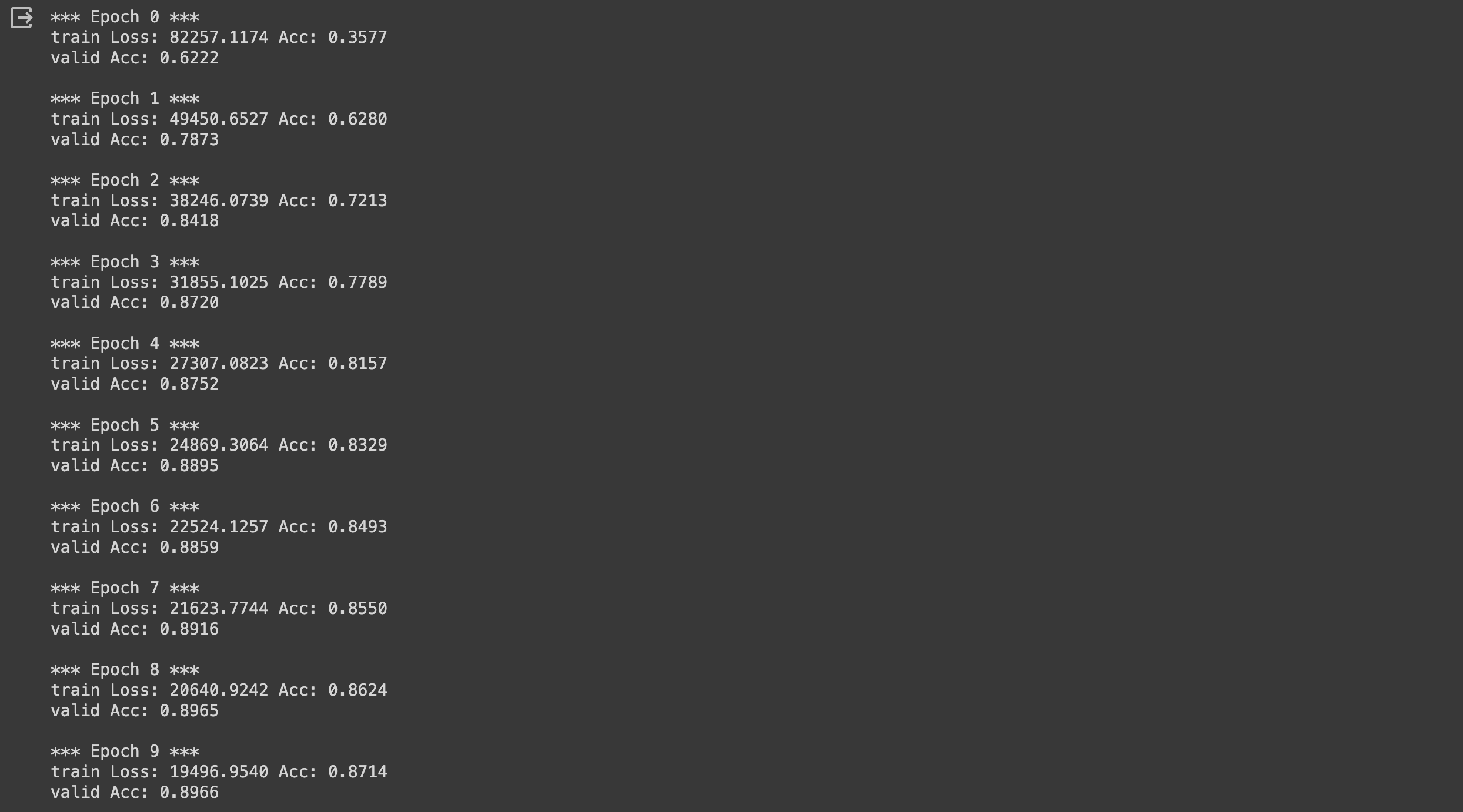
그러고나서 test dataset으로 test를 해봤을 때의 결과는 아래와 같이 나왔다.
model.eval()
running_acc = 0.0

for idx, (inputs, labels) in enumerate(dataloaders_test):
  inputs = inputs.to(device)
  labels = labels.to(device)

  with torch.set_grad_enabled(False):
    outputs, _ = model(inputs)
    _, preds = torch.max(outputs, 1)

    # statistics
    running_acc += torch.sum(preds == labels.data)
running_acc /= (idx+1) * batch_size
print('{} Acc: {:.4f}\n'.format('test', running_acc))
# test Acc: 0.8987
모델 구현을 블로그에 포스팅하는 것은 처음인데, 포스팅 때문인지 코드를 엄청 꼼꼼하게 보게 된 기회였던 것 같다. 평소에 구현이나 코드를 보는 공부를 별로 좋아하지 않아서 잘 안했는데 이번 구현 포스팅 덕분에 흥미를 조금 붙인 것 같다. 처음이라 많이 부족하지만 그래도 시작이 중요한 법! 앞으로 기회가 된다면 종종 포스팅해서 포스팅도 깔끔하게 하고 구현 실력도 늘리는 기회가 됐으면 좋겠다!!
'Experience > Naver Boostcamp 6기' 카테고리의 다른 글
| 네이버 부스트캠프 그 후 이야기 (1) | 2024.06.20 |
|---|---|
| [최종 프로젝트 일지 - 3주차] 멘토님 피드백 준비 (0) | 2024.03.23 |
| [최종 프로젝트 일지 - 2주차] 삽질의 연속... (3) | 2024.03.14 |
| [최종 프로젝트 일지 - 1주차] 최종 프로젝트 시작! (2) | 2024.03.12 |
| [최종 프로젝트 일지 - 0주차] 쉽지 않았던 준비 기간... (0) | 2024.03.10 |


