| 일 | 월 | 화 | 수 | 목 | 금 | 토 |
|---|---|---|---|---|---|---|
| 1 | ||||||
| 2 | 3 | 4 | 5 | 6 | 7 | 8 |
| 9 | 10 | 11 | 12 | 13 | 14 | 15 |
| 16 | 17 | 18 | 19 | 20 | 21 | 22 |
| 23 | 24 | 25 | 26 | 27 | 28 | 29 |
| 30 | 31 |
- Programmers
- transformer
- 네이버 부스트캠프 ai tech 6기
- rectified flow
- video editing
- 3d generation
- diffusion
- diffusion models
- BOJ
- DP
- 코테
- segmenation map generation
- emerdiff
- diffusion model
- Vit
- segmentation map
- dreammotion
- masactrl
- 프로그래머스
- VirtualTryON
- video generation
- 3d editing
- visiontransformer
- 코딩테스트
- flow matching
- image editing
- Python
- score distillation
- inversion
- 논문리뷰
- Today
- Total
평범한 필기장
[평범한 학부생이 하는 논문 리뷰] Flow Matching For Generative Modeling (ICLR 2023) 본문
[평범한 학부생이 하는 논문 리뷰] Flow Matching For Generative Modeling (ICLR 2023)
junseok-rh 2025. 2. 7. 04:58Paper : https://arxiv.org/abs/2210.02747
Flow Matching for Generative Modeling
We introduce a new paradigm for generative modeling built on Continuous Normalizing Flows (CNFs), allowing us to train CNFs at unprecedented scale. Specifically, we present the notion of Flow Matching (FM), a simulation-free approach for training CNFs base
arxiv.org
(성민혁 교수님 강의 자료 참고 : https://www.youtube.com/watch?v=B4FfBNKl2tg&t=1296s)
Abstract

본 논문에서는 Flow Matching(FM)을 제안함 → fixed conditional probability path의 vector field를 이용해서 CNF를 학습하는 방식임.
1. Introduction
기존의 Diffusion model의 한계점
학습 + 샘플링이 오래 걸림. 효율적인 샘플링을 위해서는 특정 매서드(DDIM sampling)을 적용해야함.
Continuous Normalizing Flow
임의의 probability path를 모델링할 수 있고 특히 diffusion process에 의해 모델링된 probability path를 통합할 수 있다고 알려짐.
문제 : 학습이 어려움. →ODE를 풀어야하는데, time-consuming함.
Flow Matching
CNF 모델을 학습시키는 효율적인 simulation-free approach. → CNF training을 supervise하는 일반적인 probability path의 선택을 허용함.
Flow Matching Objective : 원하는 probability path를 생성하는 target vector field에 대해 regression
Conditional Flow Matching : per-example training objective, 동일한 gradient를 제공, intractable target vector field에 대한 명시적인 knowledge가 필요 없음.
⇒ Diffusion path에 대해서도, FM을 사용하면 더 robust하고 stable한 학습이 가능하다. + score matching보다 더 좋은 performance를 보임.
2. Preliminaries : Continuous Normalizing Flows
- Probability density path : $p_t$ → time dependent probability density function
- Time dependent vector field : $v_t$
- Flow map : $\phi_t$ → ODE를 통해 $v_t$로 정의
- $\phi_0(x) = x$
- $\frac{d}{dt} \phi_t(x) = v_t(\phi_t(x))$
Normalizing Flow
- reference distribution $p_0(x_0)$을 target distribution $p_1(x_1)$로 옮기는게 목적 ($\phi$를 이용해서, $x_0 \sim p_0, x_1 = \phi(x_0)$)
- 확률 밀도 보존 법칙(??)을 만족해야함 → $p_1(x_1)dx_1 = p_0(x_0)dx_0$ ⇒ $dx_0 = \vert \mathrm{det}(\frac{\partial \phi^{-1}(x_1)}{\partial x_1}) \vert$

- push forward operator $[ \phi ]*$ : $p_1(x_1) = p_0(\phi^{-1}(x_1))\vert \mathrm{det}(\frac{\partial \phi^{-1}(x_1)}{\partial x_1}) \vert = [\phi]*p_0(x_1)$ → 분포를 옮기는 연산자 느낌
- Objective Function : $\mathcal{L} = -\mathbb{E}{x_1 \sim p_1} \mathrm{log}([\phi\theta]_*p_0(x_1))$
- Challenge : $\phi^{-1}$와 Jacobian을 계산해야함
Residual Flow
- $\phi_t(x_t) = x_t + \Delta_t \cdot u_t(x_t)$
- Residual Flow 부분을 continuous로 변경

- Fokker-Planck Equation
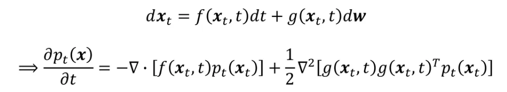
- $\frac{dx_t}{xt} = u_t(x_t)$일 때, 위 식을 변형하면,
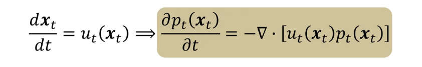
- 결국 아래처럼 식 변형
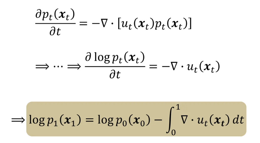
- Objective function : $\mathcal{L} = -\mathbb{E}{x_1 \sim p_1} \mathrm{log}p_1(x_1)$ → $\phi\theta(x_0)$대신 vector field $u_\theta(x_t,t)$를 학습함
- 문제 : ODE를 풀어야하는데 이건 time consuming
3. Flow Matching
- Reference Distribution : $p_0 \sim \mathcal{N}(x\vert 0, I)$
- Target Distribution : $p_1 \approx q$
Data distribution $q$를 알 수 없으니까 $p_1$를 통해 approximate하려함.
또, CNF에서 vector field를 알면 $p_0 \rightarrow p_1$가 가능해서 Flow matching objective를 그런 방식으로 디자인함.
Target probability density path $p_t(x)$와 이에 대응되는 vector field $u_t(x)$가 주어지면 다음과 같이 Flow Matching objective를 정의할 수 있음
$\mathcal{L}{FM}(\theta) = \mathbb{E}{t,p_t(x)} \Vert v_t(x) - u_t(x) \Vert^2$
근데, $p_t, u_t$를 모르기 때문에 intractable하다.
3.1 Constructing $p_t, u_t$ from Conditional Probability Paths and Vector Fields
Target probability path를 구성하는 간단한 방식은 simpler probability path의 mixture를 이용하는 것.
Data sample $x_1$이 주어졌을 때, $p_t(x|x_1)$는 conditional probability path를 나타냄.
- $t=0$일 때, $p_0(x|x_1)=p(x)$를 만족
- $t=1$일 때, $p_1(x|x_1)$는 $x=x_1$에 집중된 분포로 디자인($p_1(x|x_1) = \mathcal{N}(x|x_1,\sigma^2I)$, 여기서 $\sigma>0$는 충분히 작음)
Marginal probability path는 conditional probability path를 $q(x_1)$에 대해 marginalize해서 다음과 같이 나타냄.

$t=1$일 때, $p_1$은 다음과 같고 $q$를 approximate함.

Marginal vector field를 다음과 같이 conditional vector field를 marginalize함으로써 정의할 수 있음
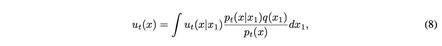
이 방식으로 conditional vector field를 aggregate하는 것은 marginal probability path를 모델링하기 위한 정확한 vector field를 야기한다.
- (8) 식은 conditional vector field를 가중합하면 marginal vector field가 된다는 것을 나타냄.
- 여기서 가중치는 $\frac{p_t(x|x_1)q(x_1)}{p_t(x)} = \frac{p_t(x|x_1)q(x_1)}{\int p_t(x|x_1)q(x_1)dx_1}$로 전체에서 $x_1$의 비율을 나타내고 이에 대해 $x_1$에서의 vector field를 모든 $x_1$을 가중합이라고 이해 가능!
Key Observation

이를 통해 unknown & intractable marginal VF를 간단한 conditional VF로 분해. → 위처럼 single data sample에 의존하는 것처럼 간단하게 정의.
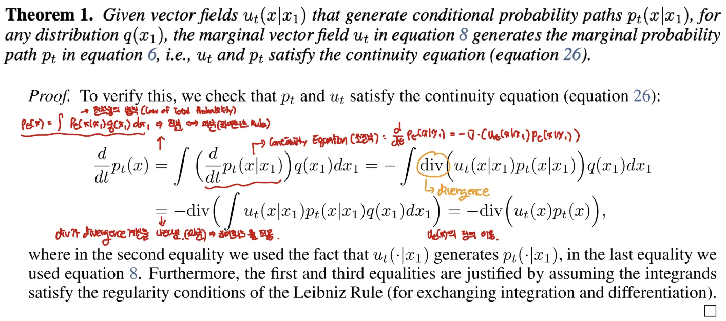
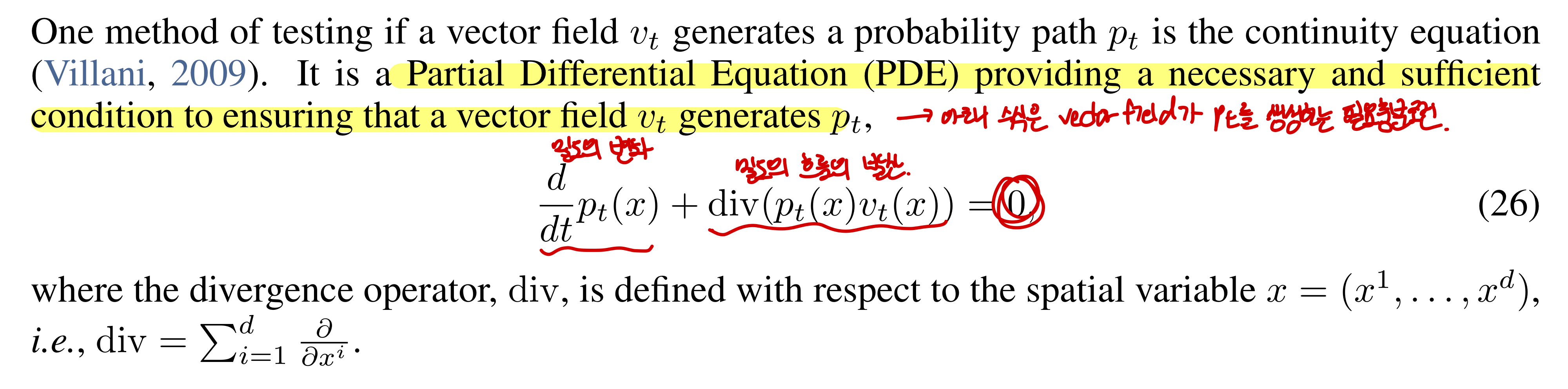
Continuity equation은 vector field $v_t$가 $p_t$를 생성하는 필요충분 조건. 증명에서 continuity equation을 만족하니까 marginal vector field는 marginal probability path를 생성.
3.2 Conditional Flow Matching
수식 (6),(8)에서의 marginal probability path랑 marginal VF의 정의에서 integral은 intractable.
→ $u_t$가 여전히 intractable
이 때문에 naive하게 original Flow Matching objective의 unbiased estimator 계산하는 것은 intractable.
더 간단한하지만 original objective와 동일한 optima를 보이는 objective를 제안(Conditional Flow Matching)

Key Observation

CFM objective를 optimize하는 것은 FM objective를 optimize하는 것과 동일함
→ Marginal probability path나 marginal vector field를 계산하지 않고 CNF를 학습시켜 marginal probability path $p_t$를 생성 가능.
적절한 conditional probability path와 vector field만 디자인하면 됨
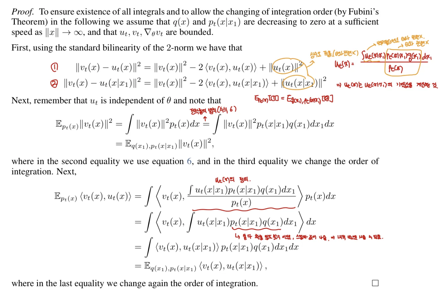
$\mathcal{L}_{CFM},\mathcal{L}_{FM}$의 기댓값을 구했을 때, $u_t(x), u_t(x|x_1)$가 $\theta$와 independent한데 이 부분 제외하고는 같음
→ 그러므로 $\nabla_\theta \mathcal{L}_{FM}(\theta) = \nabla_\theta \mathcal{L}_{CFM}(\theta)$
4. Conditional Probability Paths and Vector Fields
(Conditional vector field와 conditional probability path를 디자인을 어떻게 하느냐에 대해 설명)
Conditional Flow Matching objective는 conditional probability path와 conditional vector field에 대한 어떤 선택과도 작동함.
Conditional probability path가 다음과 같음.

여기서 $\mu_0(x_1)=0, \sigma_0(x_1)=1$라고 셋팅. → 모든 conditional probability path가 $t=0$에서는 $p(x) = \mathcal{N}(x|0,I)$인 동일한 Standard Gaussian noise distribuiton으로 converge.
$\mu_1(x_1) = x_1, \sigma_1(x_1)=\sigma_{min}$로 셋팅해서 $p_1(x|x_1)$가 $x_1$을 중심으로한 완전 좁은 gaussian 분포가 되게 함.
Flow map은 다음 형태를 고려함.

$\psi_t$는 noise distribution $p_0(x|x_1) = p(x)$를 $p_t(x|x_1)$로 push.

이 flow는 conditional probability path를 생성하는 vector field를 제공함

$x_0$에 대해서 $p_t(x|x_1)$를 reparameterize하고 수식 (13)을 넣으면 CFM loss는 다음과 같아짐.
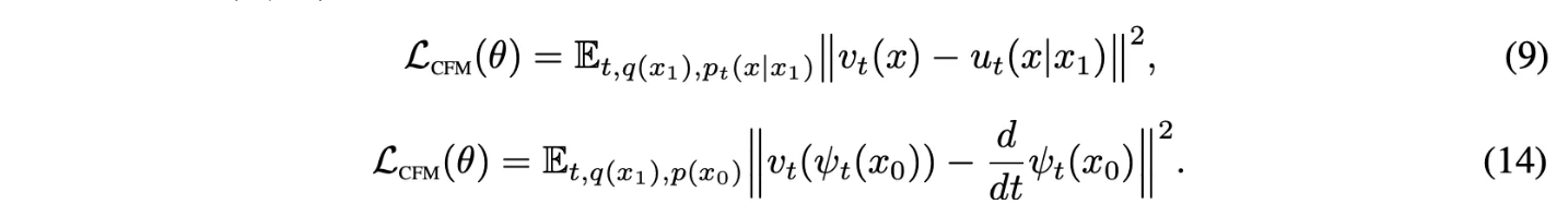
- $x = \psi_t(x_0) = \sigma_t(x_1)x_0 + \mu_t(x_1)$
- 원래 $v_t$가 $u_t(x|x_1)$를 학습하는데, 수식 (13)을 이용해 변경 가능
→ $\psi_t$를 알면 vector field를 알 수 있음.
→ $\psi_t$를 학습하면 돼~
→ 효율성과 단순성을 위해서 저렇게 수식 10, 11처럼 정의(GPT왈)
요약하면 10, 11처럼 정의하면 conditional vector fieldf를 구할 수 있고, 이걸로 CFM을 학습 가능
4.1 Special Instances of Gaussian Conditional Probability Paths
논문의 formulation은 임의의 함수 $\mu_t(x_1), \sigma_t(x_1)$에 대해서 fully general함
Desired boundary conditions를 만족하는 어떤한 differentiable function으로도 셋팅 가능
Example I : Diffusion conditional VFs
Reversed(noise→data) Variance Exploding path

- $\sigma_0 = 0, \sigma_1 \gg 1$
- $\mu_t(x_1) = x_1, \sigma_t(x_1) = \sigma_{1-t}$
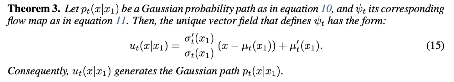
Theorem 3에 넣으면 아래와 같음

Reversed Variance Preserving path

- $\beta$는 noise scale function
- $\mu_t(x_1) = \alpha_{1-t}x_1,\sigma_t(x_1) = \sqrt{1-\alpha^2_{1-t}}$
Theorem 3에 넣으면 다음과 같음

본 논문의 conditional VF $u_t(x|x_1)$은 실제로 deterministic probability flow에 사용된 vector field와 일치 (이러한 conditional diffusion process로 제한했을 때)
Diffusion conditional VF를 Flow Matching objective와 결합하는 것은 attractive training alternative 제공 → 더 stable하고 robust
Diffusion process에서의 probability path들은 완전한 true noise distribution에 도달하지 않음(in finite time)
본 논문의 construction은 probability path를 완전히 control하고 직접 $u_t, \sigma_t$ 셋팅하기 때문에 그렇지 않음.
Example II : Optimal Transport conditional VFs
Mean과 std를 time에 대해 linear하게 정의

Theorem 3에 의해서 VF는 다음과 같음

모든 $t \in [0,1]$에서 정의.
$u_t(x|x_1)$에 대응되는 conditional flow는 다음과 같음

이 경우에 CFM loss는 다음과 같음

Mean과 std가 linear하게 변하도록 하는 것은 simple하고 intuitive path를 야기함
Conditional flow $\psi_t(x)$가 실제로 두 Gaussian $p_0(x|x_1), p_1(x|x_1)$사이의 Optimal Transport displacement map임
OT interpolant가 다음처럼 정의 되는데, 여기서 $(1-t)\mathrm{id} + t\psi$를 OT displacement map이라함.

본 논문에서는 수식 (22)가 OT displacement map이 됨
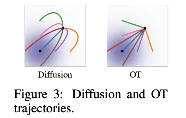
OT displacement map하에서 particle들은 항상 직선으로 일정한 속도로 움직임
5. Experiments
5.1 Density Modeling and Sampling Quality on ImageNet
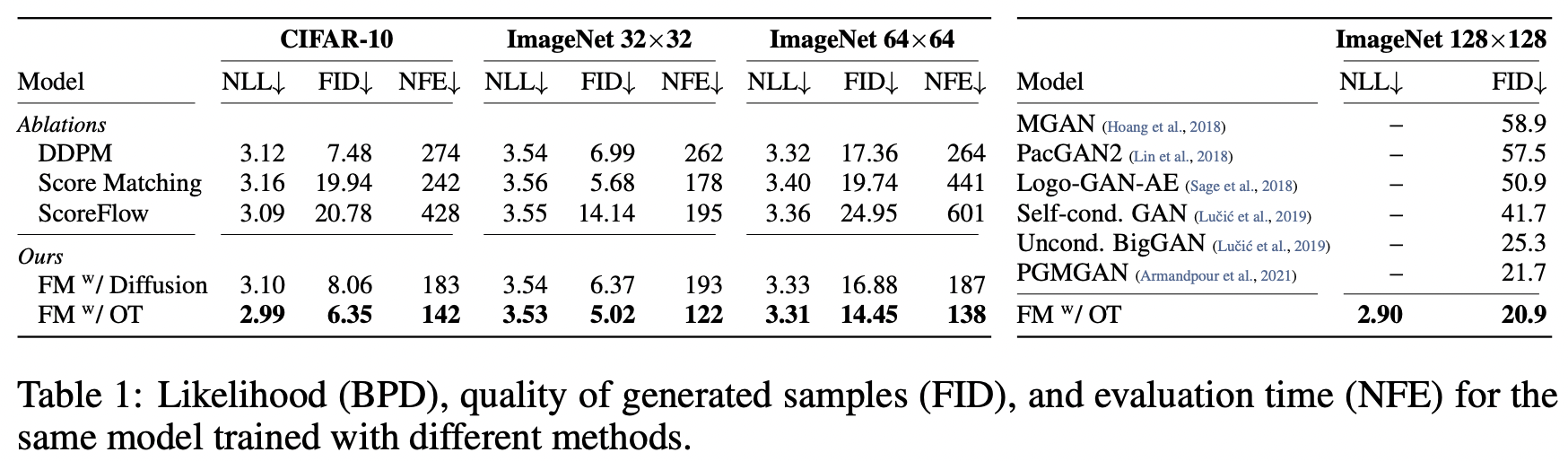
Faster training
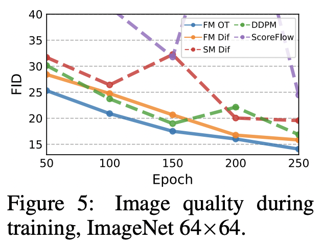
Flow Matching이 일반적으로 더 빠르게 수렴
5.2 Sampling Efficiency
a random noise sample $x_0 \sim \mathcal{N}(0,I)$그리고 학습된 VF $v_t$로 ODE solver를 가지고 (1)을 풀어서 $\phi_1(x_0)$를 계산함
Diffusion model은 SDE formulation을 통해 샘플링되는데, 이는 매우 비효율적임
동일한 computational cost에 대해서 lower error를 발생시켜 ODE solver가 더 효율적이기 때문
OT path로 Flow Matching을 사용해서 학습된 model은 항상 ODE solver에 상관없이 가장 efficient sampler 가져옴
Sample paths
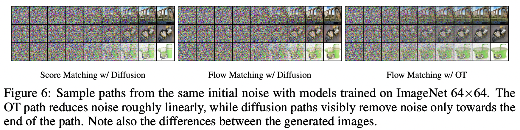
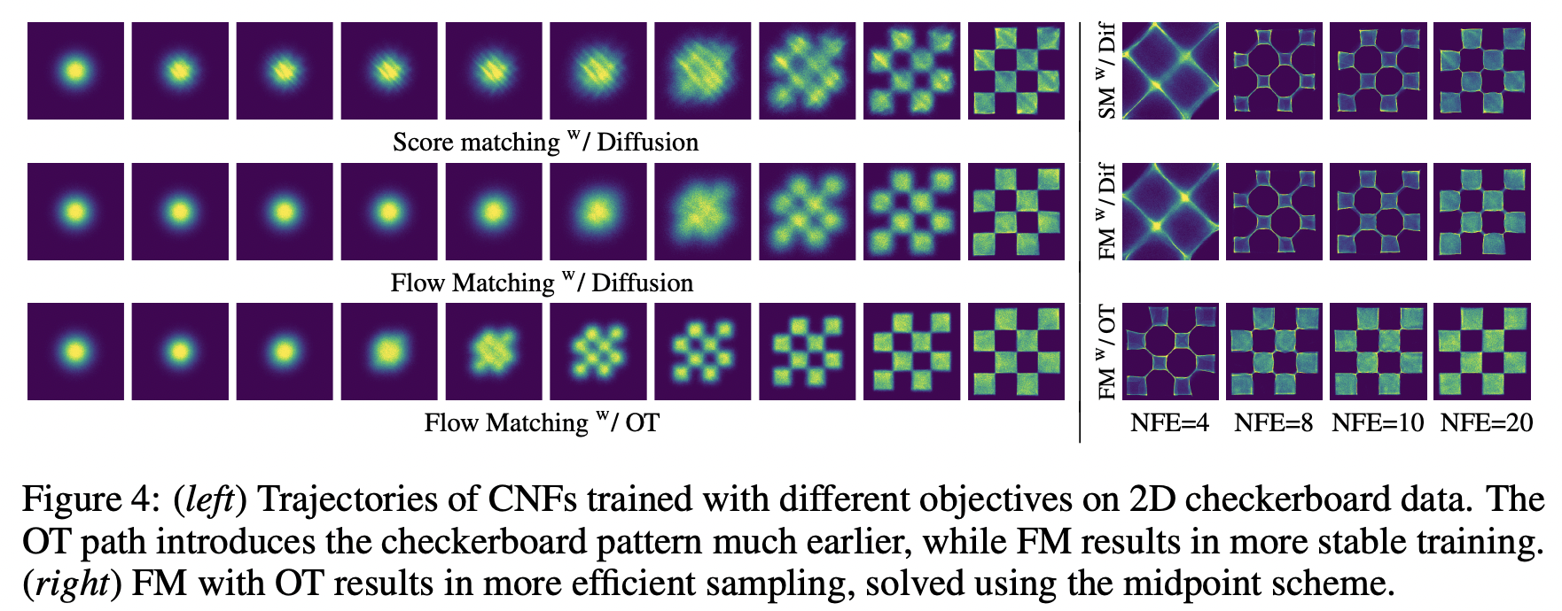
OT path를 사용할 때 diffusion path보다 더 이르게 이미지를 생성하기 시작.
Low-cost samples
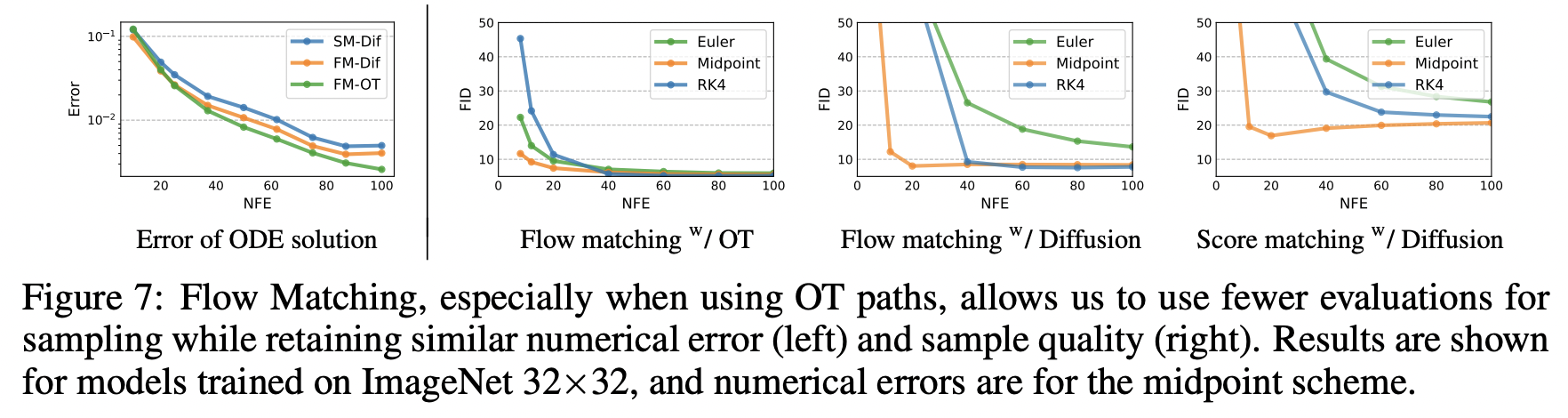
FM with OT가 가장 좋은 numerical error를 보임. → 60%의 NFE로 diffusion model과 동일한 error threshold에 도달
FM with OT가 매우 작은 NFE값에서 FID 감소를 달성
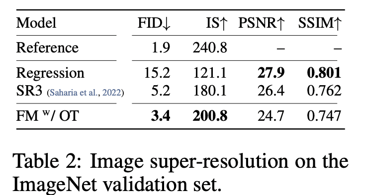
5.3 Conditional Sampling from Low-Resolution Images