
| 일 | 월 | 화 | 수 | 목 | 금 | 토 |
|---|---|---|---|---|---|---|
| 1 | 2 | 3 | 4 | 5 | 6 | 7 |
| 8 | 9 | 10 | 11 | 12 | 13 | 14 |
| 15 | 16 | 17 | 18 | 19 | 20 | 21 |
| 22 | 23 | 24 | 25 | 26 | 27 | 28 |
- Programmers
- ddim inversion
- flow matching models
- VirtualTryON
- BOJ
- rectified flow
- 네이버 부스트캠프 ai tech 6기
- Python
- visiontransformer
- rectified flow models
- 3d editing
- diffusion
- unlearning
- image editing
- image generation
- diffusion models
- video generation
- 프로그래머스
- rectified flow matching models
- 논문리뷰
- video editing
- 코테
- flow models
- memorization
- 3d generation
- Concept Erasure
- diffusion model
- flow matching
- inversion
- Machine Unlearning
- Today
- Total
평범한 필기장
[평범한 학부생이 하는 논문 리뷰] Diffusion Models Beat GANs on Image Synthesis 본문
[평범한 학부생이 하는 논문 리뷰] Diffusion Models Beat GANs on Image Synthesis
junseok-rh 2024. 4. 10. 00:261. Introduction
기존 diffusion models는 LSUN과 ImageNet과 같은 어려운 generation에서는 GAN (BIgGAN-deep)에 경쟁이 되지 않는 FID score를 냈다. 본 논문에서 diffusion models와 GANs사이의 차이는 (1) 최신 GAN의 architecture는 고도로 연구되고 refine되었다는 것과 (2) GANs는 다양성을 fidelity로 맞바꿀 수 있다는 것이다. 본 논문에서는 이 두 가지의 이점을 가져오는 것을 목표로 한다. (1)은 모델 아키텍쳐를 향상시킴으로써 (2)는 다양성을 fidelity로 맞바꾸는 계획을 구상함으로써 해결하려한다. 이를 통해 몇 개의 metric과 dataset에서 GAN을 뛰어넘는 sota를 달성했다고 한다.
2. Background
2.1 Improvements
Background에서 DDPM, NCSN, Improved DDPM 논문에 대해 간단하게 설명하고 있다.
https://juniboy97.tistory.com/46
[평범한 학부생이 하는 논문 리뷰] Denoising Diffusion Probabilistic Models (DDPM)
이번에 리뷰할 논문은 그 유명한! DDPM! Diffusion의 기초 논문들은 확실하게 이해하고 넘어가는 것이 좋다는 멘토님의 조언에 따라 이번 ddpm도 시간은 오래 걸리겠지만 최대한 꼼꼼하게 읽어서 자
juniboy97.tistory.com
https://juniboy97.tistory.com/45
[평범한 학부생이 하는 논문 리뷰] Generative Modeling by Estimating Gradients of the Data Distribution (NCSN)
이번에는 Diffusion에 제대로 도전해보자! 하는 마인드로 Diffusion 논문들도 블로그에 올리기로 다짐했다. 그래서 첫 논문으로 NCSN을 들고 왔다. 스터디해보면서 엄청 벽을 느낀 논문들이지만 다시
juniboy97.tistory.com
Improved DDPM은 아직 읽어보지는 않았지만 이 섹션에서 어느정도 설명한 부분을 참고해서 정리해보자면 DDPM에서 $\Sigma_\theta(x_t,t)$를 고정하는 것은 더 적은 diffusion 스텝으로 sampling을 할 때 sub-optimal이기에, output $v$를 다음과 같이 보간하는 신경망으로 $\Sigma_\theta(x_t, t)$를 파라미터화할 것을 제안한다.
$$\Sigma_\theta(x_t,t) = exp(v{\rm log}\beta_t + (1-v){\rm log}\tilde{\beta}_t)$$
($\beta_t$와 $\tilde{\beta}_t$는 reverse process variance의 upper와 lower)
또한, $\epsilon_\theta(x_t,t)$와 $\Sigma_\theta(x_t,t)$를 동시에 학습시키는 하이브리드 objective $L_{simple} + \lambda L_{vlb}$를 제안한다. 이를 이용하면 샘플 퀄리티를 떨어뜨리지 않고 더 적은 steps를 통해 sampling을 할 수 있다고 한다. 그래서 본 논문에서 이러한 기법들을 사용한다고 한다.
https://arxiv.org/abs/2102.09672
Improved Denoising Diffusion Probabilistic Models
Denoising diffusion probabilistic models (DDPM) are a class of generative models which have recently been shown to produce excellent samples. We show that with a few simple modifications, DDPMs can also achieve competitive log-likelihoods while maintaining
arxiv.org
본 논문에서 50 이하의 sampling step을 사용할 때, DDIM sampling을 사용한다고 한다.
2.2 Sample Quality Metrics
본 논문의 base metric은 FID score이고, fidelity를 측정할 때는 Precision 이나 IS를, diversity나 distribution coverage를 측정할 때는 Recall을 사용한다고 한다.
- Precision : data manifold에서 model sample이 차지하는 비율
- Recall : sample manifold에서 data sample이 차지하는 비율
3. Architecture Improvements
이 섹션에서는 아래와 같은 다양한 모델 architecture에 대한 ablation을 실행했다.
- 폭에 비해 깊이를 늘리고 모델 크기를 상대적으로 일정하게 유지
- Attention head 수를 늘리기
- Attention을 16 * 16에만 사용하는 대신, 32 * 32, 16 * 16, 8 * 8에 사용하기
- BigGAN residual block 사용하기
- Residual connection을 $\frac{1}{\sqrt{2}}$로 rescaling하기

위 결과를 보면 rescaling residual block을 제외하고는 모든 것들이 performance를 향상시켰다.

위 이미지를 보면 depth를 늘리는 것은 성능은 향상시키지만, training 시간을 늘리고 wider model의 성능과 동등해지는데 더 많은 시간이 든다. 그렇기에 이는 앞으로의 실험에서 쓰지 않았다고 한다.
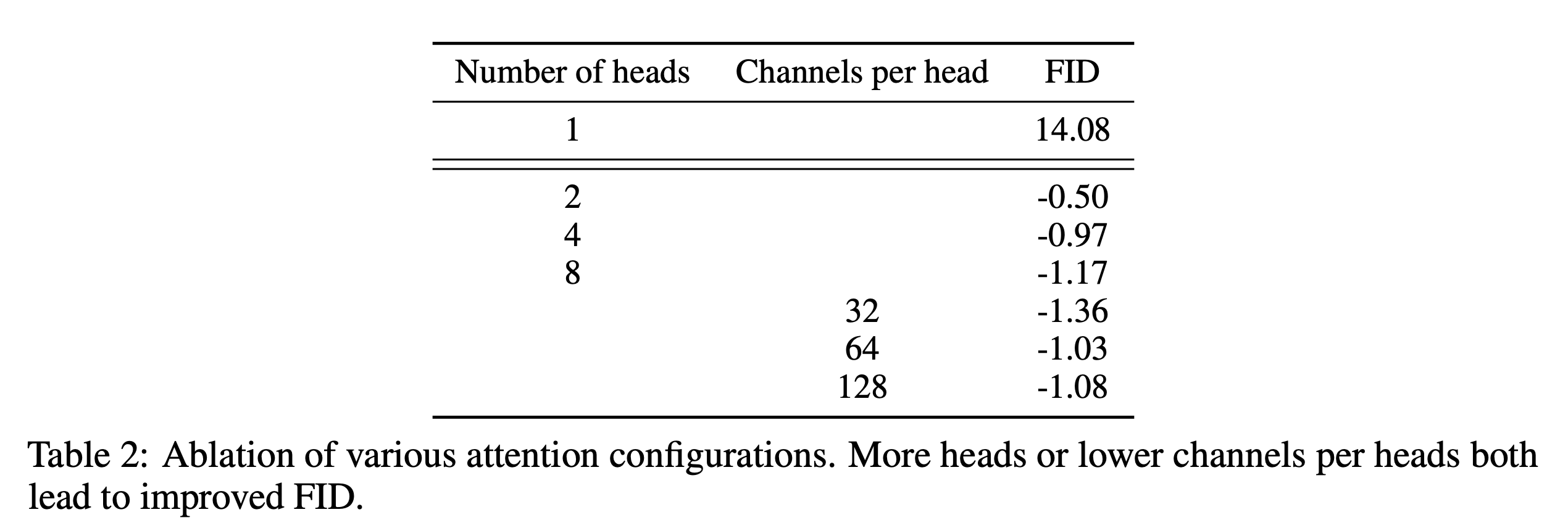
위는 attention heads를 고정하거나 channels per head 수를 고정해서 진행한 실험의 결과이다. 더 많은 attention heads나 head당 더 적은 channel는 FID score를 향상시켰다. Figure 2에서 64 channel이 시간에 대한 성능이 좋았기에 default로 64 channels per head를 사용한다.
3.1 Adaptive Group Normalization
본 논문에서는 각 residual block에 group normalization을 수행한 후에 timestep과 class embedding을 포함하기 위해 AdaGN(adaptive group normalization)을 도입한다.
$${\rm AdaGN}(h,y) = y_s{\rm GroupNorm}(h) + y_b$$
여기서 $h$는 residual block에서 convolution을 거치고 나온 결과물이다. 코드 상에서 아래 결과로 나온 $h$를 나타내는 듯 했다.
self.in_layers = nn.Sequential(
            normalization(channels),
            nn.SiLU(),
            conv_nd(dims, channels, self.out_channels, 3, padding=1),
        )
self.h_upd = Upsample(channels, False, dims)
self.x_upd = Upsample(channels, False, dims)


in_rest, in_conv = self.in_layers[:-1], self.in_layers[-1]
h = in_rest(x)
h = self.h_upd(h)
x = self.x_upd(x)
h = in_conv(h)
$y = [y_s, y_b]$는 timestep과 class embedding의 linear projection을 통해 얻어진다.

위 ablation을 통해 AdaGN이 효과가 있는 것을 알 수 있기 때문에, AdaGN을 default로 사용한다.
최종적으로 본 논문에서는 아래의 아키텍쳐를 사용한다

4. Classifier Guidance
GANs는 conditional image synthesis를 하기 위해 class labels를 많이 사용한다. Class-conditional normalization statistics의 형태를 띄거나 classifier $p(y|x)$처럼 행동하도록 명시적으로 디자인된 heads를 가진 discriminators의 형태를 띈다.
이러한 점들로부터 diffusion generator를 향상시키기 위해 classifier $p(y|x)$를 이용하는 접근 방식을 본 논문에서 탐구했다. 이전 연구들에서 classifier의 gradient를 사용하여 pre-train된 diffusion model이 conditioned될 수 있다는 것을 보였다. 이 섹션에서 classifier를 이용한 conditional sampling process 두 가지를 리뷰하고 본 논문에서 어떻게 classifier를 이용해 실제로 sample quality를 향상시켰는지 보인다.
4.1 Conditional Reverse Noising Process
Unconditional reverse noising process $p_\theta(x_t|x_{t+1})$를 label $y$에 대해 condition하기 위해, 아래와 같은 수식에 따른 각 transition으로부터 sample을 뽑는 것으로 충분하다.

이 분포로부터 샘플을 뽑는 것은 intractable하지만 perturbed Gaussian distribution을 통해 근사화될 수 있다.

위 결과 수식에서 $C_4$는 (2)수식에서 normalizing constant $Z$와 대응되기 때문에 무시할 수 있다. 이를 통해 conditional transition operator가 unconditional transition operator와 유사한 평균이 $\Sigma g$만큼 이동한 Gaussian으로 근사화될 수 있다. 아래는 상응하는 sampling algorithm을 나타낸다.

4.2 Conditioning Sampling for DDIM
위의 conditioning sampling은 stochastic diffusion sampling에서만 가능하다. DDIM과 같은 deterministic 방식에는 적용될 수 없다. Diffusion models와 score matching사이의 connection을 이용한 sde diffusion 논문에서 적용된 score-based conditioning trick을 본 논문에서 사용했다고 한다. 샘플에 추가된 noise를 예측하는 $\epsilon_\theta(x_t)$가 있다고 하면, 이를 이용해 아래의 score function을 유도할 수 있다.

좌변은 NCSN에서 $s_\theta(x_t)$로 근사되고, 이는 DDPM에서 $\epsilon_\theta(x_t)$앞에 우변과 같은 상수가 붙은 것과 같은 것으로 기억해 (11)번 식이 나오는 것으로 이해했다. 본 논문은 $p(x_t)p(y|x_t)$의 score function으로 대체했다.

$p(x_t,y) = p(x_t)p(y|x)$에 대한 score에 대응하는 새로운 epsilon prediction $\hat{\epsilon}(x_t)$을 본 논문에서 아래와 같이 정의한다.

$\hat{\epsilon}(x_t)$를 이용해 DDIM에서 사용한 동일한 sampling procedure를 이용한다.

4.3 Scaling Classifier Gradients
본 논문에서 ImageNet에 학습된 분류모델을 이용해 classifier guidance를 적용했다. Classifier architecture는 8*8 layer에 attention pool을 적용한 UNet모델의 downsampling trunk으로 되어있다. 그리고 이 classifier는 diffusion model과 동일한 noising distribution에 대해 학습시킨다. 또한 overfitting을 줄이기 위해 random crops를 더했다. 수식 (10)을 이용해 diffusion model의 sampling process에 classifier가 포함된다.
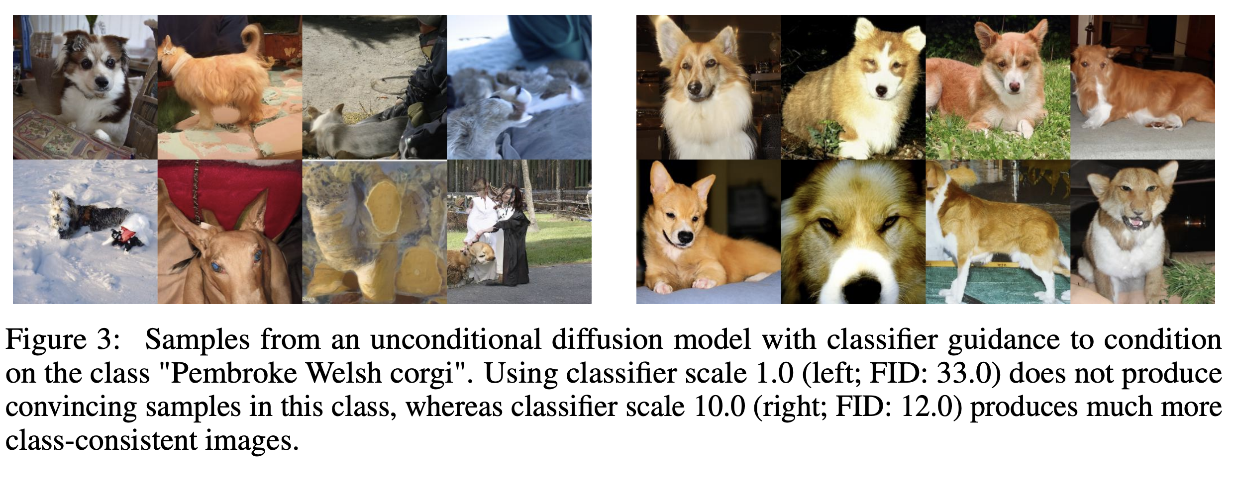
Unconditional ImageNet models로 한 초기 실험에서, 1보다 큰 constant factor로 classifier gradients를 scale할 필요가 있다는 것을 발견했다. 1로 scale을 할 때, final sample들에 대해 classifier가 적절한 확률(약 50%)를 할당하지만, 육안으로 봤을 때는 의도한 class와 매칭되지 않는 것을 확인했다. Classifier gradient를 scale up하면 이러한 문제를 해결하고 class probability가 100% 근처까지 나온다고 한다.
Scaling classifier gradients의 효과를 이해하기 위해,
$$s \cdot \nabla_x{\rm log}p(y|x) = \nabla_x {\rm log} \frac{1}{Z}p(y|x)^s$$
를 봐보자. 여기서 $Z$는 임이의 상수이다. 결과적으로, conditional process는 $p(y|x)^s$에 비례하는 re-normalized classifier distribution에 이론적으로 기초된다. $s > 1$이면, 이 분포는 $p(y|x)$보다 더 sharp해진다. 즉, 더 큰 gradient scale을 사용하는 것은 classifier의 mode에 더 집중하고, (덜 다양하지만) 더 높은 fidelity를 가진 sample을 생성하기에 더 바람직하다.
위에서 unconditional diffusion model (modeling $p(x)$)을 가정했지만, conditional diffusion model ($p(x|y)$)을 학습시키는 것 또한 가능하다. Classifier guidance를 동일한 방식으로 사용한다. 아래의 표는 classifier guidance의 영향을 나타낸 결과이다.

5. Results

5.1 State-of-the-art Image Synthesis
위 이미지는 논문의 결과를 요약해 놓은 표이다. FID에서는 각 task에서 가장 좋은 점수를 얻었고, sFID에서는 하나의 task 제외하고 가장 좋은 점수를 얻었다. 개선된 architecture로만 LSUN과 ImageNet 64*64에서 이미 sota를 달성했다. 더 고해상도의 ImageNet에 대해, classifier guidance는 best GANs를 능가하게 했다는 것을 관찰했다. 이러한 모델들은 recall에 의해 측정된 것처럼 높은 분포에 대한 coverage를 유지하면서 GANs와 유사한 perceptual quality를 얻었고 심지어 25 step만으로 이를 해냈다.

위 이미지는 BigGAN-deep과 본 논문의 diffusion model의 random sample을 비교한 결과이다. 위 이미지들을 보면 diffusion model이 더 많은 mode를 포함하는 것을 볼 수 있다.
5.2 Comparision to Upsampling
이번 섹션에서는 guidance와 two-stage upsampling stack을 비교한다. Nichol and Dhariwal과 Saharia et al.에서는 low-resolution diffusion 모델과 그에 상응하는 upsampling diffusion model을 결합한 two-stage diffusion model을 학습시킨다. 샘플링 동안, low-resolution model은 이미지를 생성하고, upsampling model은 이 이미지에 condition된다. 이 방식은 ImageNet 256*256에서 FID score를 향상시켰지만 BigGAN-deep과 같은 sota만큼 도달하지는 못했다.

본 논문에서는 higher resolution으로 upsampling하기 전에 lower resolution에서 guidance를 사용하는 것으로 가장 좋은 FID를 달성했다.
6. Limitations
- 아직 GANs에 비해 sampling 속도가 느리다.
- Labeled 데이터셋에서만 사용 가능하다.


